library(quantstrat)
## Loading required package: quantmod
## Loading required package: xts
## Loading required package: zoo
##
## Attaching package: 'zoo'
## The following objects are masked from 'package:base':
##
##     as.Date, as.Date.numeric
## Loading required package: TTR
## Registered S3 method overwritten by 'quantmod':
##   method            from
##   as.zoo.data.frame zoo
## Loading required package: blotter
## Loading required package: FinancialInstrument
## Loading required package: PerformanceAnalytics
##
## Attaching package: 'PerformanceAnalytics'
## The following object is masked from 'package:graphics':
##
##     legend
## Loading required package: foreach
library(quantmod)
library(TTR)
library(purrr)
##
## Attaching package: 'purrr'
## The following objects are masked from 'package:foreach':
##
##     accumulate, when

source("./utils.R")Nofri’s Congestion Phase System
Notes taken from Trading Systems and Methods, 5th edition, Chapter 4 (p.155)
Nofri’s Congestion Phase System is a sideway market trading system. It is built on a foundation that a great part of the time in the market is in nontrending motion. The price whipsaws between a Higher bound and Lower Bound.
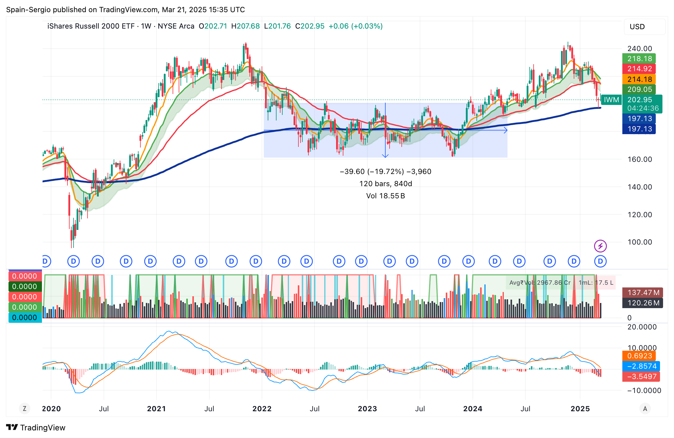
For example, in the blue-boxed period from Jan 2022 to Nov 2023, IWM is in a sideways action, until the breakout in early 2024. A trending strategy will not be able to use here as the price move sideways, and therefore we need a strategy that can adapt to sideways market.
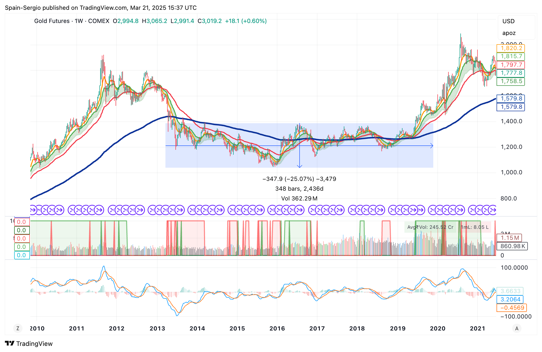
Another example is Gold futures is in a sideways market from 2013 Mar to 2019 Nov.
During sideways period, trend-following strategy will not work. The main idea of this strategy is to bring steady small profits during this period, while waiting for the trending period resumes.
The challenge of this strategy are:
- To identify the congestion period (sideway period) - User of the Congestion Phase System need to wait to be certain of a well-defined congestion area before beginning a trading sequence.
- Position sizing and stop loss - How should that be set to ensure a positive expectancy?
- Anticipation of Breakout vs False Breakout
Implementing the strategy
Basis of the strategy
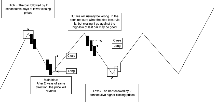
The Basis of the strategy is a 3-day reversal (事不過三原則). When in the range, we anticipate that the price will reverse after 2 consecutive days of the same direction. This strategy aims for high successfully probability but low risk-to-reward.
Implementation details
Defining Congestion Zone
We define the congestion high as the bar followed by 2 consecutive low bars (Only active if found) ✅
We define the congestion low as the bar followed by 2 consecutive high bars (Only active if found) ✅
Penetration of a previous top and formation of a new top redefine the range without altering the bottom point; the opposite case can occur for new bottoms. (Expand Range) ✅
A new high or low price cancels the congestion area ✅
If 2+ consecutive days with prices closing almost unchanged, consider as one day
Handling breakouts
If top or bottom has been formed, and followed by a major breakout or price run, wait for 10 days to find the new zone to ensure the continuance of the congestion area and limit the risk during more volatile period
Define major breakout: The “large move” was defined as any net price change (absolute value) over a 10-day interval that was at least two times larger than the average net change over 10 days for all past data. (2x 10-day Average True Range) ✅
Cancel the congestion zone and search for a new one ✅
If a false breakout occurs lasting two or three days, safety suggests a waiting period of seven days.
- Define false breakout: If there is a breakout (above or below congestion zone) but return to original congestion zone within 2 days, it is a false breakout.
Entry
Entry long position on the next day if 2-day down
Entry short position on the next day if 2-day up
Exit
Position will be closed everyday if taken.
Variation: Stop loss on yesterday’s high
Implementation and backtesting using quantstrat
The following section will implement the strategy and backtest it by using the quantstrat library. We will use 10 years of daily data for the following universe.
Equity:
US: IYY, SPY, QQQ, IWM
Asia: FXI, EWJ, VNM, INDA, EWY, EWT
Europe: EWQ, EWI, EWG, EWU
South America: ARGT, EWW, EWZ
Emerging markets: ACWX, EEM
Bonds: SHY(1-3 years TBond), TLT (20+ Year Treasury Bond)
Commodities: GC, SI, HG, CL, NG, HO, RB, CT, ZC, ZS, ZL, ZW, SB
Forex: 6A, 6B, 6C, 6E, 6J, 6S, 6N, DX
To learn more on Quantstrat, this series of blogs are great intro:
https://quantstrattrader.com/2014/09/09/nuts-and-bolts-of-quantstrat-part-i/
https://quantstrattrader.com/2014/09/16/nuts-and-bolts-of-quantstrat-part-ii/
https://quantstrattrader.com/2014/09/20/nuts-and-bolts-of-quantstrat-part-iii/
https://quantstrattrader.com/2014/09/24/nuts-and-bolts-of-quantstrat-part-iv/
https://quantstrattrader.com/2017/04/13/nuts-and-bolts-of-quantstrat-part-v/
# Setup quantstrat
Sys.setenv(TZ = "UTC")
currency('USD')
## [1] "USD"

# Setup Dates
init_date <- "2015-01-01"
start_date <- "2015-03-15"
end_date <- "2025-03-15"

# Setup trade size and initial equity
init_equity <- 1e4 # $10,000
unit_risk   <- init_equity * 0.01
adjustment <- TRUE

symbols <- c(
  "IWM", # iShares Russell 2000 Index ETF
  "QQQ", # PowerShares QQQ TRust, Series 1 ETF
  "SPY", # SPDR S&P 500 ETF Trust
  "FXI",
  "EWJ",
  "VNM",
  "INDA",
  "EWY",
  "EWT",
  "EWQ",
  "EWI",
  "EWG",
  "EWU",
  "ARGT",
  "EWW",
  "EWZ",
  "ACWX",
  "EEM",
  "SHY",
  "TLT",
  "GLD",
  "SLV",
  "CPER",
  "USO"
)
# Note: `getSymbols()` is from `quantmod`
getSymbols(Symbols = symbols,
src = "yahoo",
index.class = "POSIXct",
from = start_date,
to = end_date,
adjust = adjustment)
## [1] "IWM" "QQQ" "SPY" "FXI" "EWJ" "VNM" "INDA" "EWY" "EWT" "EWQ"
## [11] "EWI" "EWG" "EWU" "ARGT" "EWW" "EWZ" "ACWX" "EEM" "SHY" "TLT"
## [21] "GLD" "SLV" "CPER" "USO"
stock(symbols, currency = "USD", multiplier = 1)
## [1] "IWM" "QQQ" "SPY" "FXI" "EWJ" "VNM" "INDA" "EWY" "EWT" "EWQ"
## [11] "EWI" "EWG" "EWU" "ARGT" "EWW" "EWZ" "ACWX" "EEM" "SHY" "TLT"
## [21] "GLD" "SLV" "CPER" "USO"chartSeries(Ad(SPY), type="line", theme = "white.mono", line.type = "l", bar.type="hlc")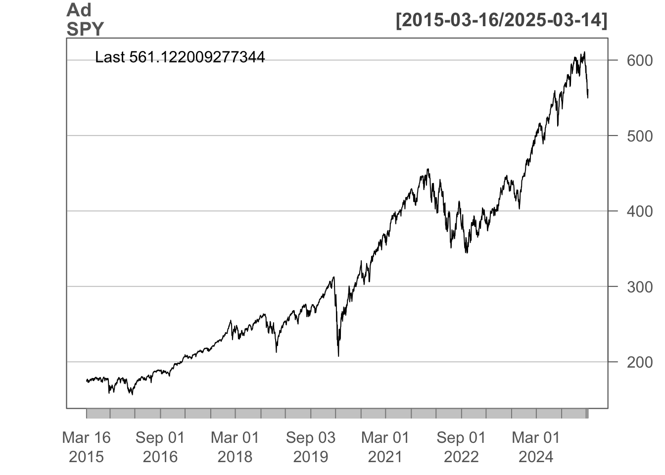
Initialise quantstrat Account, Portfolio, and Strategy
# Naming Account, Portfolio, and Strategy
# One account can contain more than one portfolio
# One portfolio can contain more than one strategy
strategy.st <- portfolio.st <- account.st <- "nofri-strat"
# Remove any existing strategy
rm.strat(strategy.st)

# Initialise Portfolio
initPortf(portfolio.st,
          symbols = symbols,
          initDate = init_date,
          currency = "USD")
## [1] "nofri-strat"

# Initialise Account
initAcct(account.st,
         portfolios = portfolio.st,
         initDate = init_date,
         currency = "USD",
         initEq = init_equity)
## [1] "nofri-strat"

# Initialise Order book
initOrders(portfolio.st,
           initDate = init_date)

# Initialise the strategy
strategy(strategy.st,
         store = TRUE)
Developing indicators
For this strategy, we have to develop the following indicators:
A congestion zone high and low price level
An indicator to indicate there is 2 lower closes in a row. This indicate the bar before the 2 lower closes is a potential congestion high.
An indicator to indicate there is 2 higher closes in a row. This indicate the bar before the 2 lower closes is a potential congestion low.
An indicator to indicate Congestion High is Active
An indicator to indicate Congestion Low is Active
ATR to determine break out
A new high indicator and a new low indicator
Indicators are transformation of market data. Indicators gain smoothness from market data, but it incurs a lag penalty compared to raw data (Trade-off between clarity and responsiveness)
Indicators attempt to paint a clearer picture of what occurs in price movements of the asset under analysis, but it needs to look at past data, which means it may not be reacting quickly with real-time data.
Another way to think about indicators is like applying an indicator by using apply() in R to the time series. You pass in the name of a function along with arguments, and then label it.
Here are the 5 steps to develop the indicator
Write the
add.indicator()functionSupply the strategy name (e.g.
strategy.st)Name the function for calculating the indicator (e.g.
SMA). This will be an important step to understand the Time series under the hood.Supply the inputs for the function as a list
Provide a label to your indicator
add.indicator(strategy = strategy.st,
              name = "SMA",
              arguments = list(x = quote(Cl(mktdata)), n = 200),
              label = "SMA200")
After developing the indicator, you can test it out by using applyIndicators() to see the immediate results:
test <- applyIndicators(strategy = strategy.st, mktData = OHLC(SPY))
head(test)
tail(test)source("./indicators.R")add.indicator(strategy = strategy.st,
name = "ATR",
arguments = list(HLC = quote(HLC(mktdata)), n = 10),
label = "ATR")
## [1] "nofri-strat"
add.indicator(strategy = strategy.st,
name = "newHigh",
arguments = list(x = quote(Cl(mktdata))),
label = "newHigh")
## [1] "nofri-strat"
add.indicator(strategy = strategy.st,
name = "newLow",
arguments = list(x = quote(Cl(mktdata))),
label = "newLow")
## [1] "nofri-strat"
add.indicator(strategy = strategy.st,
name = "diff_rel_atr",
arguments = list(data = quote(mktdata)),
label = "diff_atr_10")
## [1] "nofri-strat"
add.indicator(strategy = strategy.st,
name = "breakout_ind",
arguments = list(data = quote(mktdata),
ATRx_threshold = 2,
direction_up = TRUE),
label = "upward")
## [1] "nofri-strat"
add.indicator(strategy = strategy.st,
name = "breakout_ind",
arguments = list(data = quote(mktdata),
ATRx_threshold = 2,
direction_up = FALSE),
label = "downward")
## [1] "nofri-strat"
add.indicator(strategy = strategy.st,
name = "consecutive_ind",
arguments = list(data = quote(mktdata), n = 2),
label = "2_bar_lower")
## [1] "nofri-strat"
add.indicator(strategy = strategy.st,
name = "consecutive_ind",
arguments = list(data = quote(mktdata), op = `>`, n = 2),
label = "2_bar_higher")
## [1] "nofri-strat"
add.indicator(strategy = strategy.st,
name = "congestion_price_level_candidates",
arguments = list(data = quote(mktdata),
consecutive.down_ind_col = "consecutive_ind.2_bar_lower",
consecutive.up_ind_col = "consecutive_ind.2_bar_higher",
n = 2,
ATRx = 2),
label = "congestion_zone")
## [1] "nofri-strat"
add.indicator(strategy = strategy.st,
name = "dummy",
arguments = list(x = quote(Cl(mktdata))),
label = "dummy")
## [1] "nofri-strat"Develop signals
It is important to note that ALL signals are generated at market close. The action will be taken the day after.
A signal are interactions of market data and indicators, or indicators with another indicators. Signal is necessary (but not sufficient) for buy or sell order.
There are only a few signal functions:
sigComparison: Relationship between 2 indicators, returns 1 if the relationship is truesigCrossover: Similar tosigComparison, returns 1 on the first occurancesigThreshold: Compares range-bound indicator to a static quantity. It also applies the same mechanism ofsigCrossover.sigFormula: Flexible signal functions
Entry Signal
If congestion zone high and congestion zone low are both active -
sigComparison(congestionZone, 1)If 2-day consecutive higher closes / lower closes -
sigComparison(consecutiveSignal, 1)Entry long position on the next day if 2-day down
Entry short position on the next day if 2-day up
add.signal(strategy.st,
           name = "sigThreshold",
           arguments = list(column = "congestion_zone_active.congestion_zone",
                            threshold = 1,
                            relationship = "eq",
                            cross = FALSE),
           label = "congestion_zone_active_sig")
## [1] "nofri-strat"

add.signal(strategy.st,
           name = "sigThreshold",
           arguments = list(column = "consecutive_ind.2_bar_lower",
                            threshold = 1,
                            relationship = "eq",
                            cross = FALSE),
           label = "two_bar_lower_long_sig")
## [1] "nofri-strat"

add.signal(strategy.st,
           name = "sigThreshold",
           arguments = list(column = "consecutive_ind.2_bar_higher",
                            threshold = 1,
                            relationship = "eq",
                            cross = FALSE),
           label = "two_bar_higher_short_sig")
## [1] "nofri-strat"

# Combined Long Signal
add.signal(strategy.st, name = "sigFormula",

           # Specify that longfilter and longthreshold must be TRUE
           arguments = list(formula = "two_bar_lower_long_sig & congestion_zone_active_sig",
                            cross = FALSE),

           # Label it longentry
           label = "longentry")
## [1] "nofri-strat"

# Combined Short Signal
add.signal(strategy.st, name = "sigFormula",

           # Specify that longfilter and longthreshold must be TRUE
           arguments = list(formula = "two_bar_higher_short_sig & congestion_zone_active_sig",
                            cross = FALSE),

           # Label it longentry
           label = "shortentry")
## [1] "nofri-strat"

test_indicators <- applyIndicators(strategy = strategy.st, mktdata = SPY)
test_sig <- applySignals(strategy = strategy.st,
                                  mktdata = test_indicators)
Develop Trading rules
The last step is to develop trading rules based on the signals. Rules are functions used to create a transaction given you wish to make one based on a signal. In R, it is more complex than indicators and signals.
For simplicity, I will all use 4 times ATR exit from entry point to calculate the optimial size.
source("./osFuns.R")add.rule(strategy.st, name="ruleSignal",
arguments=list(sigcol="longentry",
sigval=1,
ordertype="market",
orderside="long",
replace=FALSE,
prefer="Open",
osFUN=osRiskUnitATR_ETF,
riskUnit = unit_risk, ATR_x = 4, atrCol = "atr.ATR"),
type = "enter",
label = "Entry2LONG",
path.dep = TRUE)
## [1] "nofri-strat"
add.rule(strategy.st,
name = "ruleSignal",
arguments = list(sigcol = "dummy",
sigval = 1,
orderside = "long",
ordertype = "market",
orderqty = "all",
prefer = "Open",
replace = FALSE),
type = "exit",
parent = "Entry2LONG",
label = "Exit2LONG",
path.dep = TRUE)
## [1] "nofri-strat"Setup analytics
updatePortf(portfolio.st)
## [1] "nofri-strat"
dateRange <- time(getPortfolio(portfolio.st)$summary)[-1]
updateAcct(portfolio.st,dateRange)
## [1] "nofri-strat"
updateEndEq(account.st)
## [1] "nofri-strat"
Statistics
#tradeStats
tStats <- tradeStats(Portfolios = portfolio.st, use="trades", inclZeroDays=FALSE)
tStats[,4:ncol(tStats)] <- round(tStats[,4:ncol(tStats)], 2)
knitr::kable(data.frame(t(tStats[,-c(1,2)])))| ACWX | ARGT | CPER | EEM | EWG | EWI | EWJ | EWQ | EWT | EWU | EWW | EWY | EWZ | FXI | GLD | INDA | IWM | QQQ | SHY | SLV | SPY | TLT | USO | VNM | |
|---|---|---|---|---|---|---|---|---|---|---|---|---|---|---|---|---|---|---|---|---|---|---|---|---|
| Num.Txns | 612.00 | 576.00 | 610.00 | 650.00 | 594.00 | 658.00 | 648.00 | 558.00 | 576.00 | 670.00 | 698.00 | 700.00 | 638.00 | 712.00 | 628.00 | 538.00 | 616.00 | 402.00 | 490.00 | 656.00 | 418.00 | 660.00 | 600.00 | 642.00 |
| Num.Trades | 304.00 | 285.00 | 298.00 | 322.00 | 286.00 | 325.00 | 319.00 | 276.00 | 282.00 | 328.00 | 346.00 | 347.00 | 316.00 | 352.00 | 312.00 | 263.00 | 308.00 | 201.00 | 227.00 | 322.00 | 209.00 | 329.00 | 297.00 | 312.00 |
| Net.Trading.PL | -1965.62 | -3076.44 | -1223.08 | -2260.09 | -2260.76 | -2701.88 | -1278.23 | -1829.86 | -3143.91 | -2159.93 | -3440.27 | -2317.07 | -2656.47 | -1583.28 | -1599.22 | -1732.20 | -2753.52 | -1452.16 | -1284.27 | -1959.55 | -1633.68 | -2336.73 | -2045.40 | -2915.15 |
| Avg.Trade.PL | -6.47 | -10.79 | -4.10 | -7.02 | -7.90 | -8.31 | -4.01 | -6.63 | -11.15 | -6.59 | -9.94 | -6.68 | -8.41 | -4.50 | -5.13 | -6.59 | -8.94 | -7.22 | -5.66 | -6.09 | -7.82 | -7.10 | -6.89 | -9.34 |
| Med.Trade.PL | -4.11 | -8.36 | -4.51 | -6.32 | -5.25 | -2.70 | -2.13 | -5.34 | -6.33 | -4.26 | -9.04 | -5.55 | -8.61 | -4.01 | -4.46 | -6.08 | -8.85 | -6.25 | -5.70 | -5.04 | -6.08 | -5.97 | -7.04 | -8.62 |
| Largest.Winner | 51.52 | 33.41 | 78.03 | 48.92 | 44.94 | 53.20 | 56.64 | 51.87 | 44.41 | 48.81 | 28.03 | 52.30 | 37.73 | 84.68 | 51.00 | 93.98 | 28.78 | 46.10 | 49.42 | 49.88 | 28.40 | 36.02 | 64.00 | 48.48 |
| Largest.Loser | -108.09 | -68.92 | -79.65 | -101.06 | -117.93 | -934.13 | -72.81 | -131.45 | -1084.28 | -124.37 | -85.90 | -117.96 | -58.88 | -99.07 | -82.68 | -162.00 | -59.40 | -57.55 | -67.61 | -76.23 | -55.33 | -76.69 | -54.21 | -98.37 |
| Gross.Profits | 1848.20 | 665.90 | 1866.52 | 1793.46 | 1679.02 | 1953.36 | 2284.75 | 1640.91 | 1487.48 | 1988.55 | 785.12 | 2092.82 | 948.58 | 1991.56 | 1434.64 | 1631.60 | 749.59 | 566.81 | 970.58 | 1505.71 | 606.86 | 1045.09 | 1045.89 | 910.88 |
| Gross.Losses | -3813.82 | -3742.35 | -3089.60 | -4053.56 | -3939.78 | -4655.23 | -3562.98 | -3470.77 | -4631.39 | -4148.48 | -4225.39 | -4409.89 | -3605.04 | -3574.84 | -3033.86 | -3363.80 | -3503.12 | -2018.97 | -2254.85 | -3465.26 | -2240.55 | -3381.82 | -3091.29 | -3826.03 |
| Std.Dev.Trade.PL | 23.99 | 16.83 | 21.54 | 22.97 | 25.15 | 56.57 | 23.25 | 23.90 | 67.96 | 24.37 | 16.40 | 24.00 | 16.14 | 20.37 | 18.38 | 25.33 | 15.07 | 15.08 | 17.64 | 19.33 | 15.64 | 16.18 | 16.59 | 17.52 |
| Std.Err.Trade.PL | 1.38 | 1.00 | 1.25 | 1.28 | 1.49 | 3.14 | 1.30 | 1.44 | 4.05 | 1.35 | 0.88 | 1.29 | 0.91 | 1.09 | 1.04 | 1.56 | 0.86 | 1.06 | 1.17 | 1.08 | 1.08 | 0.89 | 0.96 | 0.99 |
| Percent.Positive | 43.42 | 25.96 | 39.26 | 38.51 | 39.86 | 46.46 | 45.77 | 40.22 | 40.07 | 41.46 | 27.17 | 42.36 | 28.80 | 43.47 | 39.42 | 39.16 | 28.25 | 34.33 | 37.44 | 38.51 | 29.67 | 33.43 | 31.65 | 26.60 |
| Percent.Negative | 56.58 | 74.04 | 60.74 | 61.49 | 60.14 | 53.54 | 54.23 | 59.78 | 59.93 | 58.54 | 72.83 | 57.64 | 71.20 | 56.53 | 60.58 | 60.84 | 71.75 | 65.67 | 62.56 | 61.49 | 70.33 | 66.57 | 68.35 | 73.40 |
| Profit.Factor | 0.48 | 0.18 | 0.60 | 0.44 | 0.43 | 0.42 | 0.64 | 0.47 | 0.32 | 0.48 | 0.19 | 0.47 | 0.26 | 0.56 | 0.47 | 0.49 | 0.21 | 0.28 | 0.43 | 0.43 | 0.27 | 0.31 | 0.34 | 0.24 |
| Avg.Win.Trade | 14.00 | 9.00 | 15.95 | 14.46 | 14.73 | 12.94 | 15.65 | 14.78 | 13.16 | 14.62 | 8.35 | 14.24 | 10.42 | 13.02 | 11.66 | 15.84 | 8.62 | 8.21 | 11.42 | 12.14 | 9.79 | 9.50 | 11.13 | 10.97 |
| Med.Win.Trade | 11.70 | 7.04 | 11.64 | 13.32 | 13.59 | 10.08 | 13.36 | 13.89 | 10.77 | 12.77 | 6.27 | 12.03 | 8.84 | 10.78 | 8.47 | 12.82 | 7.56 | 6.42 | 9.15 | 8.51 | 8.88 | 7.38 | 8.35 | 8.69 |
| Avg.Losing.Trade | -22.17 | -17.74 | -17.07 | -20.47 | -22.91 | -26.75 | -20.60 | -21.03 | -27.40 | -21.61 | -16.77 | -22.05 | -16.02 | -17.96 | -16.05 | -21.02 | -15.85 | -15.30 | -15.88 | -17.50 | -15.24 | -15.44 | -15.23 | -16.71 |
| Med.Losing.Trade | -17.47 | -15.14 | -12.10 | -16.52 | -16.95 | -16.91 | -15.85 | -16.69 | -16.44 | -16.62 | -14.39 | -16.30 | -13.59 | -14.46 | -11.97 | -16.78 | -13.25 | -12.98 | -12.02 | -13.74 | -12.11 | -12.66 | -13.30 | -13.23 |
| Avg.Daily.PL | -6.42 | -10.68 | -4.01 | -6.95 | -7.61 | -8.21 | -3.95 | -6.56 | -10.92 | -6.45 | -9.86 | -6.62 | -8.33 | -4.45 | -5.09 | -6.44 | -8.94 | -7.22 | -5.24 | -5.97 | -7.82 | -7.08 | -6.82 | -9.08 |
| Med.Daily.PL | -3.87 | -8.19 | -4.14 | -6.27 | -4.35 | -2.28 | -1.75 | -5.12 | -5.82 | -3.55 | -8.79 | -5.34 | -8.54 | -3.41 | -4.41 | -5.72 | -8.85 | -6.25 | -4.12 | -4.91 | -6.08 | -5.95 | -6.40 | -8.05 |
| Std.Dev.Daily.PL | 23.92 | 16.78 | 21.30 | 22.87 | 24.73 | 56.23 | 23.07 | 23.78 | 67.27 | 24.13 | 16.36 | 23.91 | 16.08 | 20.26 | 18.33 | 25.06 | 15.07 | 15.08 | 17.04 | 19.17 | 15.64 | 16.16 | 16.52 | 17.34 |
| Std.Err.Daily.PL | 1.37 | 0.99 | 1.22 | 1.27 | 1.43 | 3.10 | 1.28 | 1.42 | 3.96 | 1.32 | 0.88 | 1.28 | 0.90 | 1.07 | 1.03 | 1.53 | 0.86 | 1.06 | 1.09 | 1.06 | 1.08 | 0.89 | 0.95 | 0.97 |
| Ann.Sharpe | -4.26 | -10.11 | -2.99 | -4.83 | -4.89 | -2.32 | -2.71 | -4.38 | -2.58 | -4.24 | -9.57 | -4.40 | -8.22 | -3.48 | -4.41 | -4.08 | -9.42 | -7.61 | -4.88 | -4.95 | -7.94 | -6.96 | -6.55 | -8.31 |
| Max.Drawdown | -2189.05 | -3095.57 | -1316.11 | -2366.30 | -2312.55 | -2930.85 | -1620.29 | -2105.66 | -3221.43 | -2303.01 | -3490.26 | -2478.92 | -2675.72 | -1689.23 | -1635.32 | -1769.92 | -2816.85 | -1515.90 | -1353.89 | -2028.61 | -1652.41 | -2348.83 | -2051.72 | -2986.43 |
| Profit.To.Max.Draw | -0.90 | -0.99 | -0.93 | -0.96 | -0.98 | -0.92 | -0.79 | -0.87 | -0.98 | -0.94 | -0.99 | -0.93 | -0.99 | -0.94 | -0.98 | -0.98 | -0.98 | -0.96 | -0.95 | -0.97 | -0.99 | -0.99 | -1.00 | -0.98 |
| Avg.WinLoss.Ratio | 0.63 | 0.51 | 0.93 | 0.71 | 0.64 | 0.48 | 0.76 | 0.70 | 0.48 | 0.68 | 0.50 | 0.65 | 0.65 | 0.72 | 0.73 | 0.75 | 0.54 | 0.54 | 0.72 | 0.69 | 0.64 | 0.62 | 0.73 | 0.66 |
| Med.WinLoss.Ratio | 0.67 | 0.47 | 0.96 | 0.81 | 0.80 | 0.60 | 0.84 | 0.83 | 0.66 | 0.77 | 0.44 | 0.74 | 0.65 | 0.75 | 0.71 | 0.76 | 0.57 | 0.49 | 0.76 | 0.62 | 0.73 | 0.58 | 0.63 | 0.66 |
| Max.Equity | 21.59 | 0.00 | 73.97 | 9.27 | 32.69 | 71.24 | 85.82 | 13.25 | 0.00 | 57.49 | 22.40 | 44.29 | 0.00 | 57.99 | 0.00 | 5.73 | 0.00 | 21.76 | 55.36 | 12.96 | 5.46 | 0.00 | 0.00 | 1.36 |
| Min.Equity | -2167.46 | -3095.57 | -1242.14 | -2357.03 | -2279.86 | -2859.61 | -1534.47 | -2092.42 | -3221.43 | -2245.52 | -3467.87 | -2434.63 | -2675.72 | -1631.24 | -1635.32 | -1764.19 | -2816.85 | -1494.14 | -1298.53 | -2015.65 | -1646.95 | -2348.83 | -2051.72 | -2985.08 |
| End.Equity | -1965.62 | -3076.44 | -1223.08 | -2260.09 | -2260.76 | -2701.88 | -1278.23 | -1829.86 | -3143.91 | -2159.93 | -3440.27 | -2317.07 | -2656.47 | -1583.28 | -1599.22 | -1732.20 | -2753.52 | -1452.16 | -1284.27 | -1959.55 | -1633.68 | -2336.73 | -2045.40 | -2915.15 |
(aggPF <- sum(tStats$Gross.Profits)/-sum(tStats$Gross.Losses))
## [1] 0.3935703
(aggCorrect <- mean(tStats$Percent.Positive))
## [1] 36.71875
(numTrades <- sum(tStats$Num.Trades))
## [1] 7166
(meanAvgWLR <- mean(tStats$Avg.WinLoss.Ratio))
## [1] 0.6525source("./indicators.R")
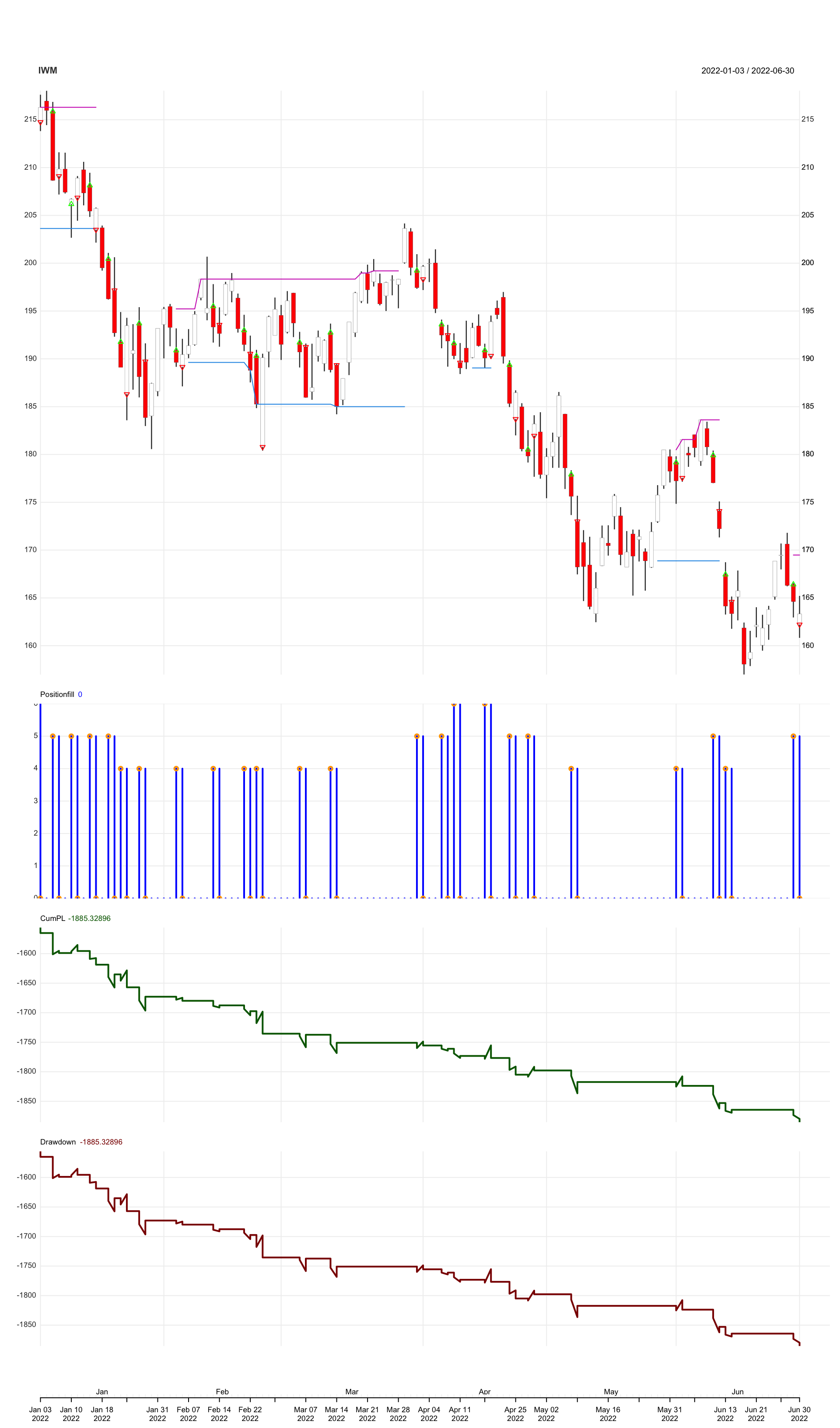
for(symbol in symbols){
indicators <- cbind(get(symbol))
indicators <- cbind(indicators, ATR(indicators, n = 10))
indicators <- cbind(indicators, newHigh(Cl(indicators)))
indicators <- cbind(indicators, newLow(Cl(indicators)))
indicators <- cbind(indicators, diff_rel_atr(indicators, atrCol = "atr"))
breakout.up <- breakout_ind(indicators, atrCol = "atr", direction_up = TRUE)
colnames(breakout.up) <- "breakout.up"
indicators <- cbind(indicators, breakout.up)
breakout.down <- breakout_ind(indicators, atrCol = "atr",
direction_up = FALSE)
colnames(breakout.down) <- "breakout.down"
indicators <- cbind(indicators, breakout.down)
consecutive_down <- consecutive_ind(indicators, op = `<`, n = 2)
colnames(consecutive_down) <- "consecutive_ind.2_bar_lower"
indicators <- cbind(indicators, consecutive_down)
consecutive_up <- consecutive_ind(indicators, op = `>`, n = 2)
colnames(consecutive_up) <- "consecutive_ind.2_bar_higher"
indicators <- cbind(indicators, consecutive_up)
congestion_zone <- cbind(indicators,
congestion_price_level_candidates(
data = indicators,
breakout.upward_ind = "breakout.up",
breakout.downward_ind = "breakout.down",
))
indicators <- cbind(indicators, congestion_zone)
congestion_high <- indicators$curr_congestion_high_price_level
congestion_low <- indicators$curr_congestion_low_price_level
newHighBool <-ifelse(indicators$newHigh == 1, TRUE, FALSE)
newLowBool <-ifelse(indicators$newLow == 1, TRUE, FALSE)
breakout.up <- ifelse(indicators$breakout.up == 1, TRUE, FALSE)
breakout.down <- ifelse(indicators$breakout.down == 1, TRUE, FALSE)
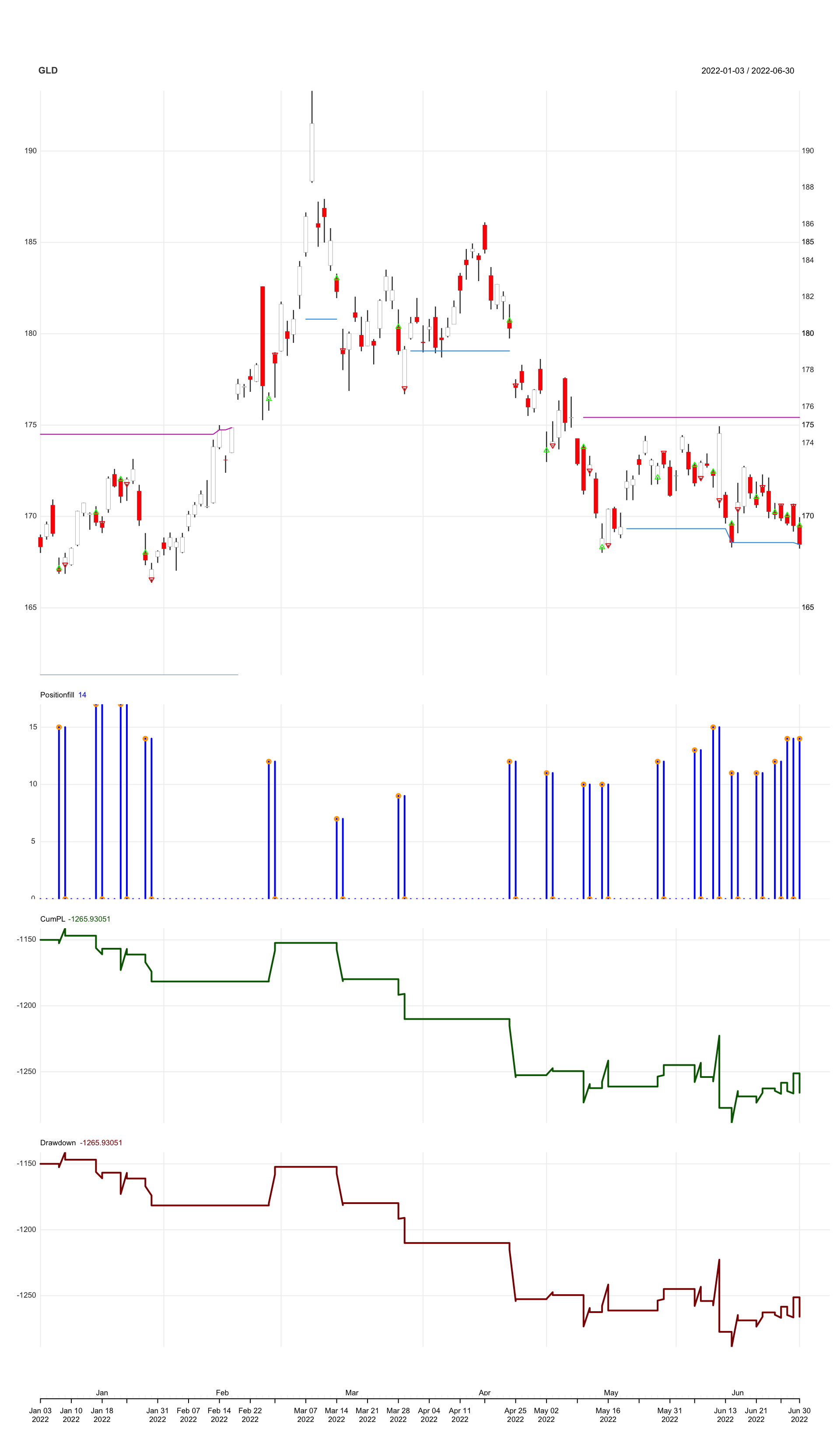
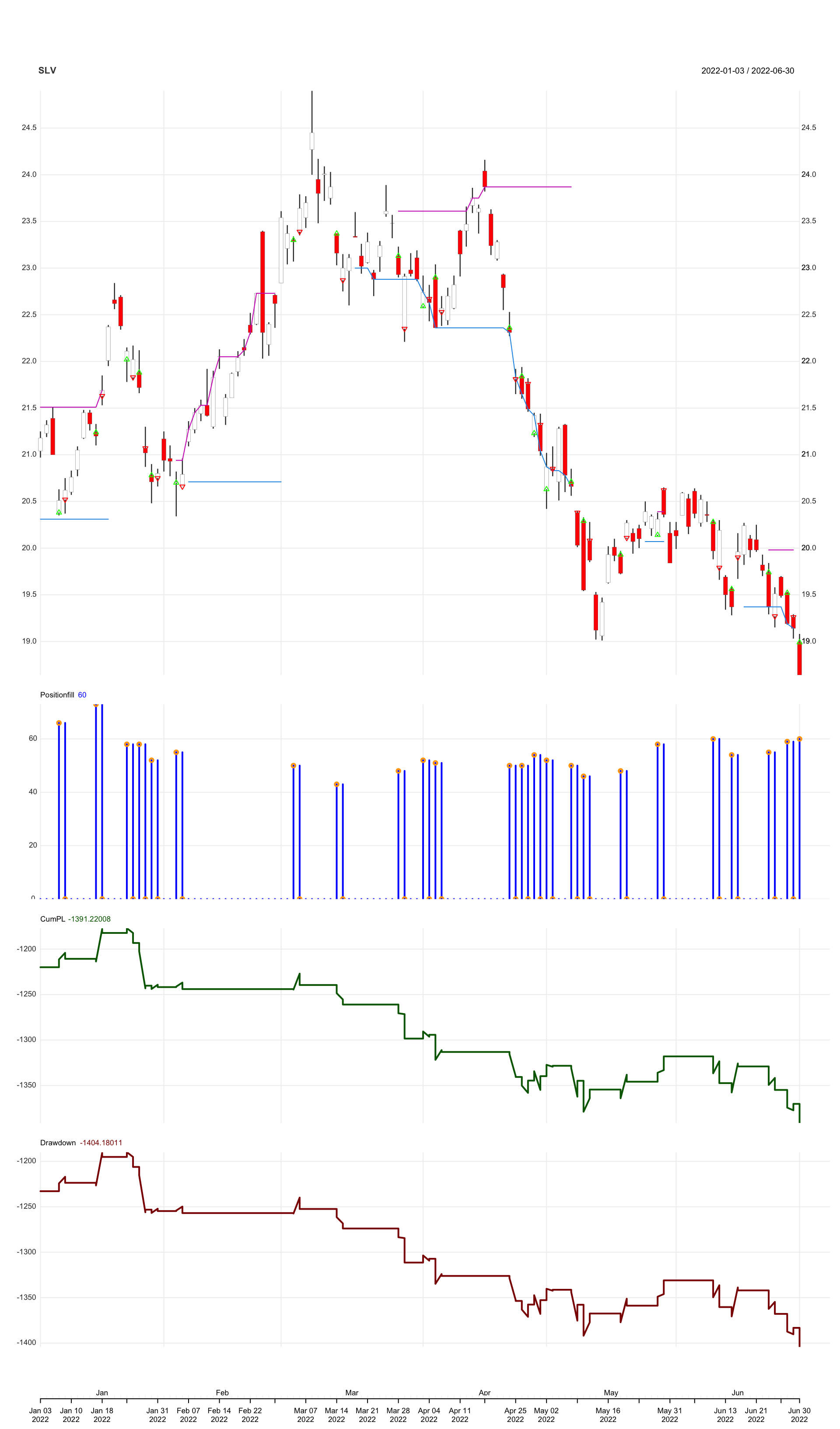
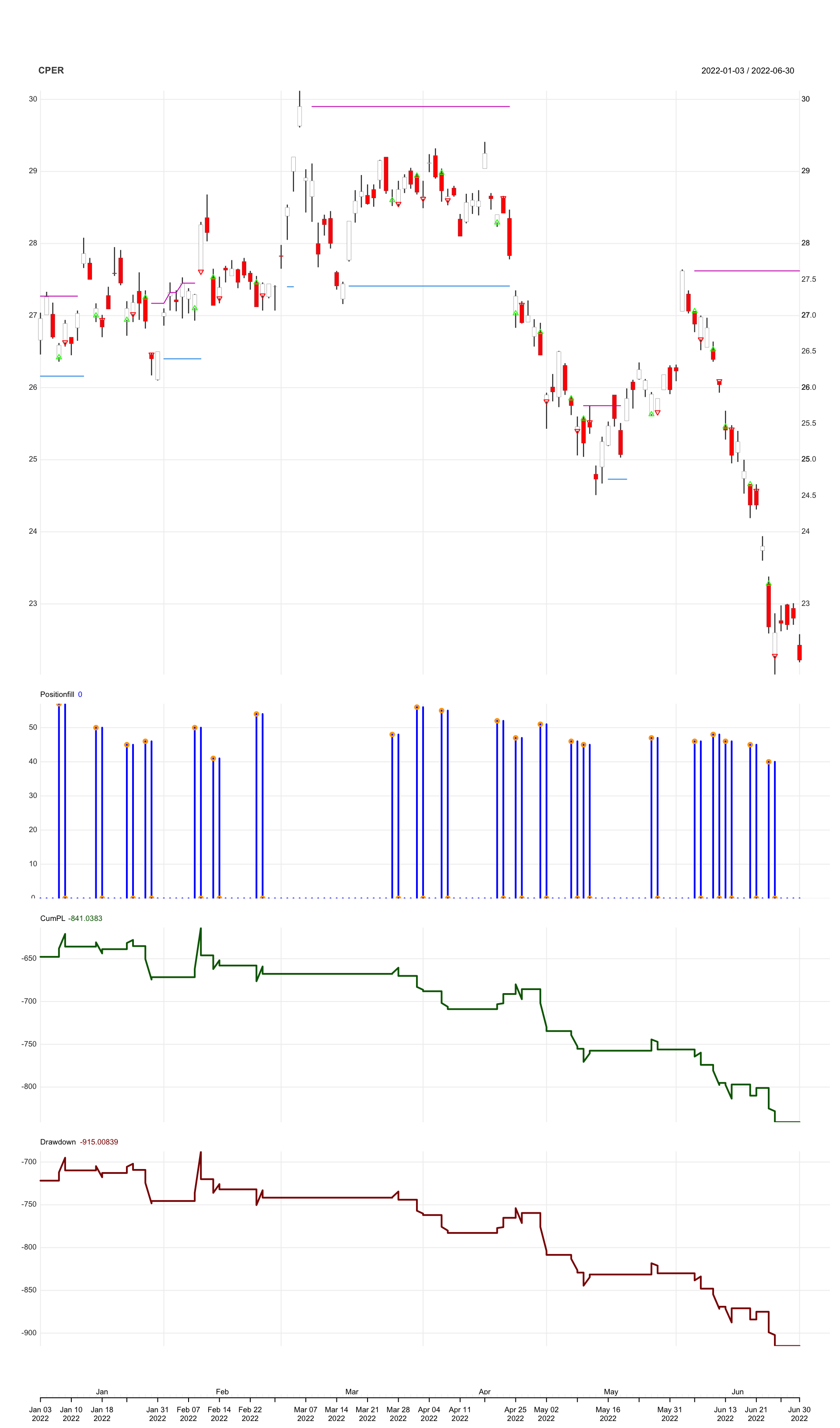
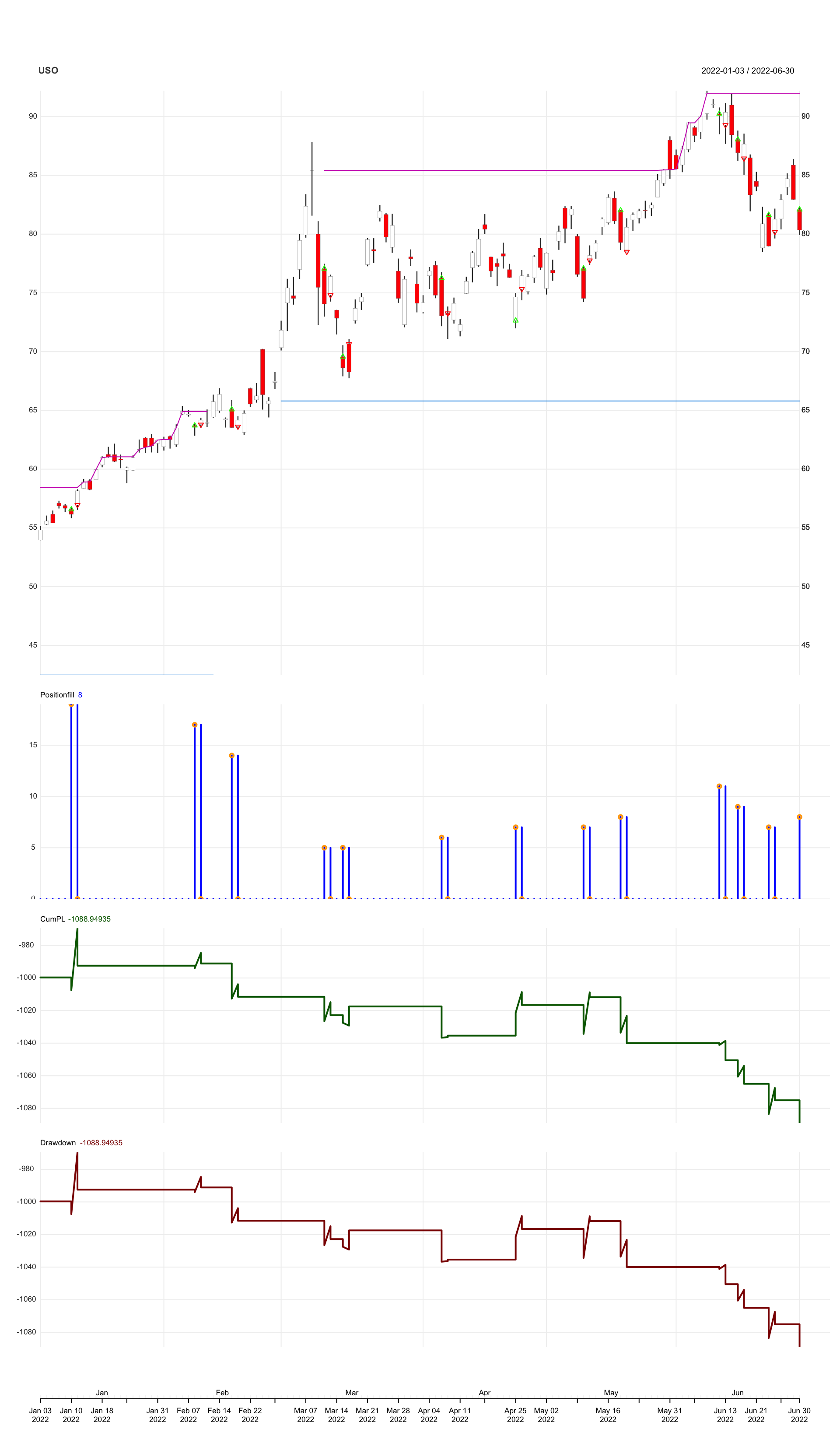
chart.Posn(Portfolio = portfolio.st,
Symbol = symbol,
subset='2022-01::2022-06',
TA = c('add_TA(congestion_high, on=1, col=6)',
'add_TA(congestion_low, on=1, col=4)'
)
)
}
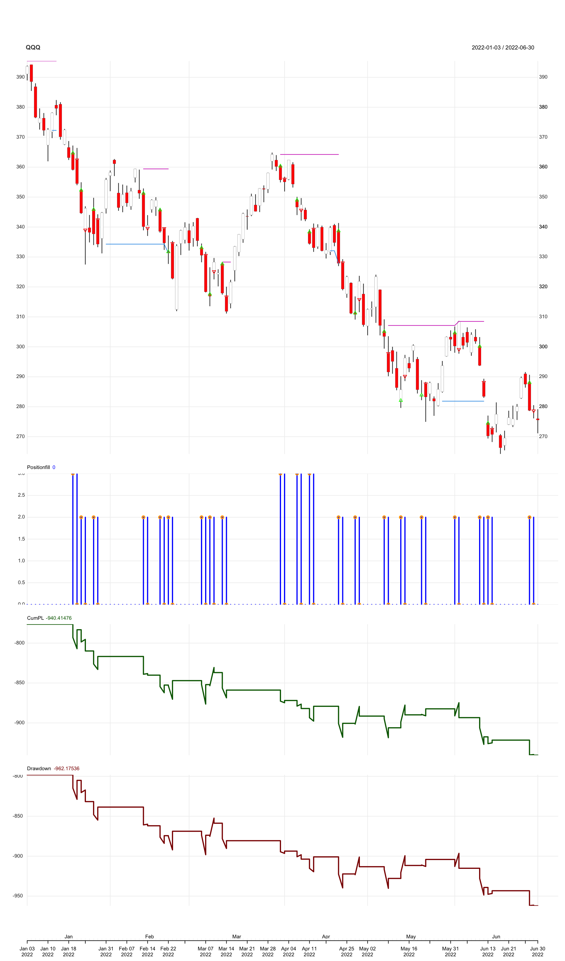
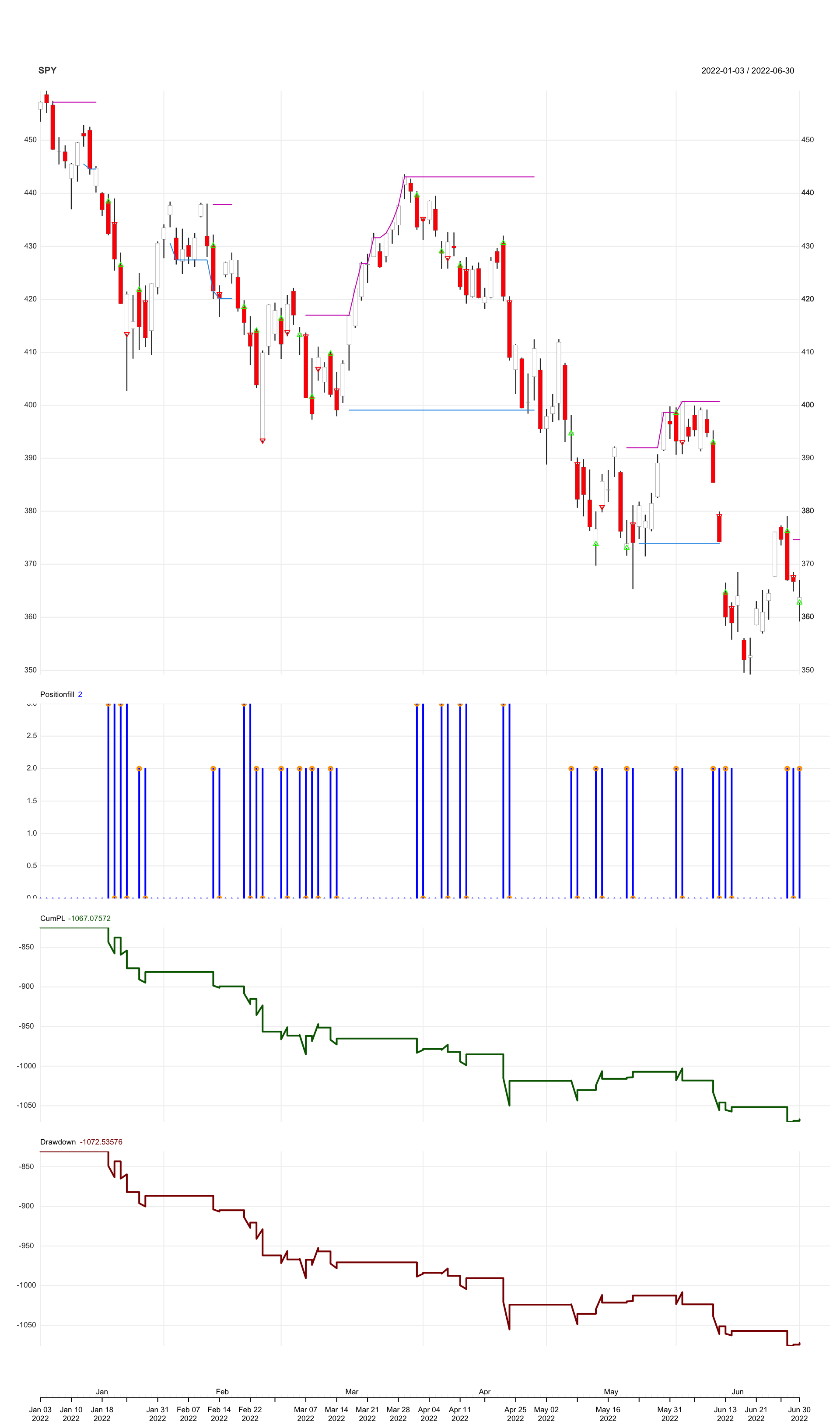
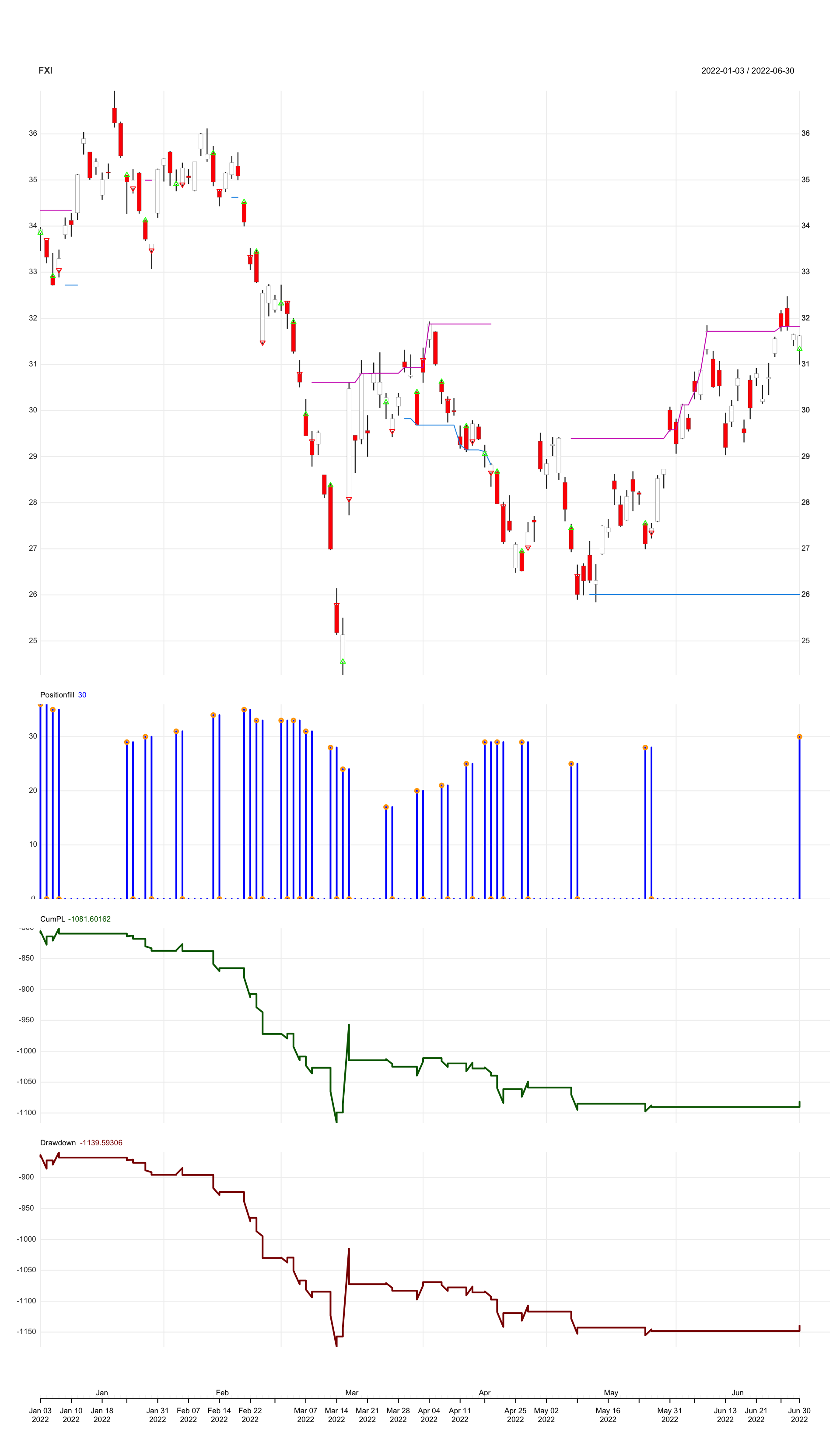
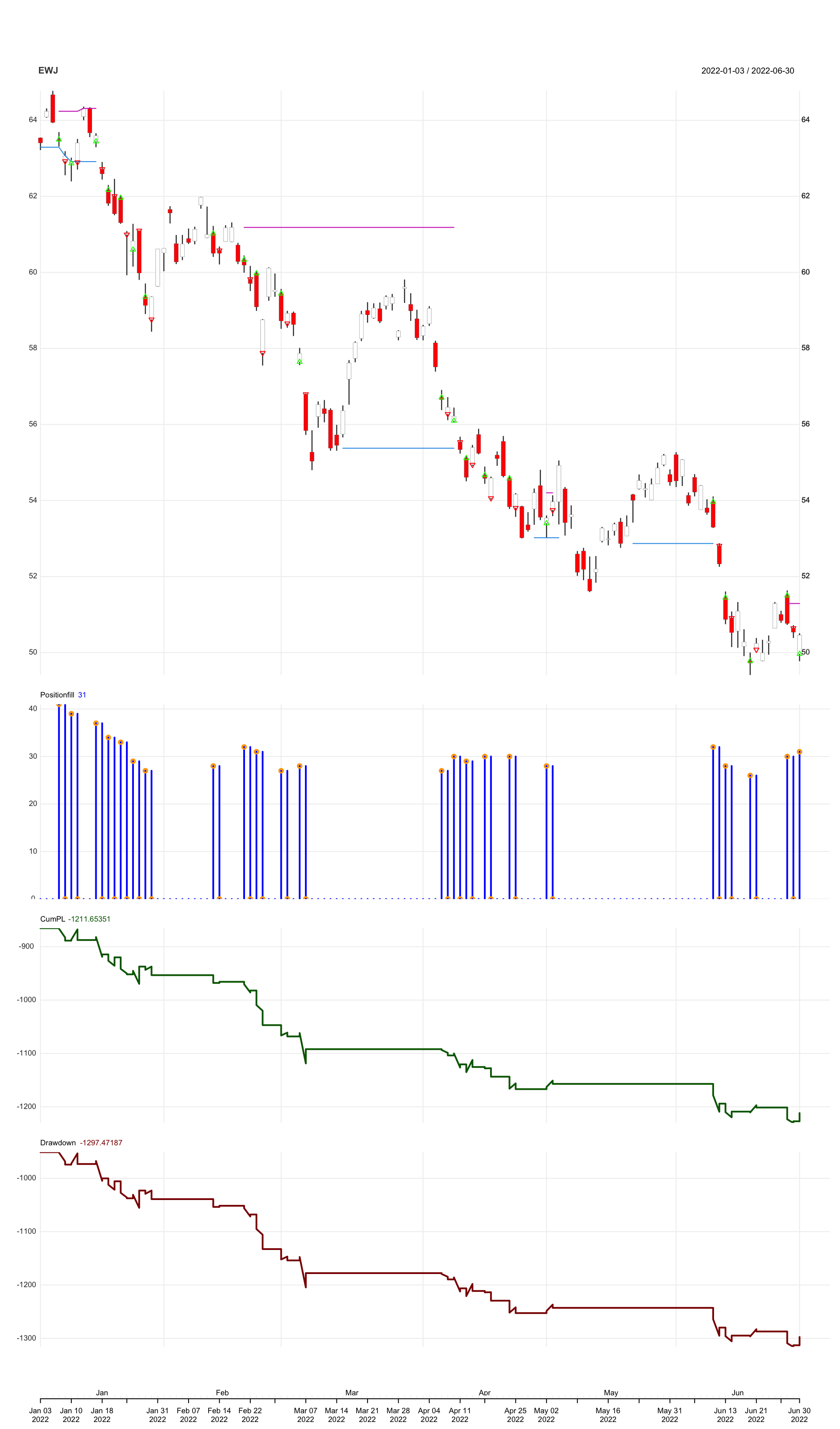
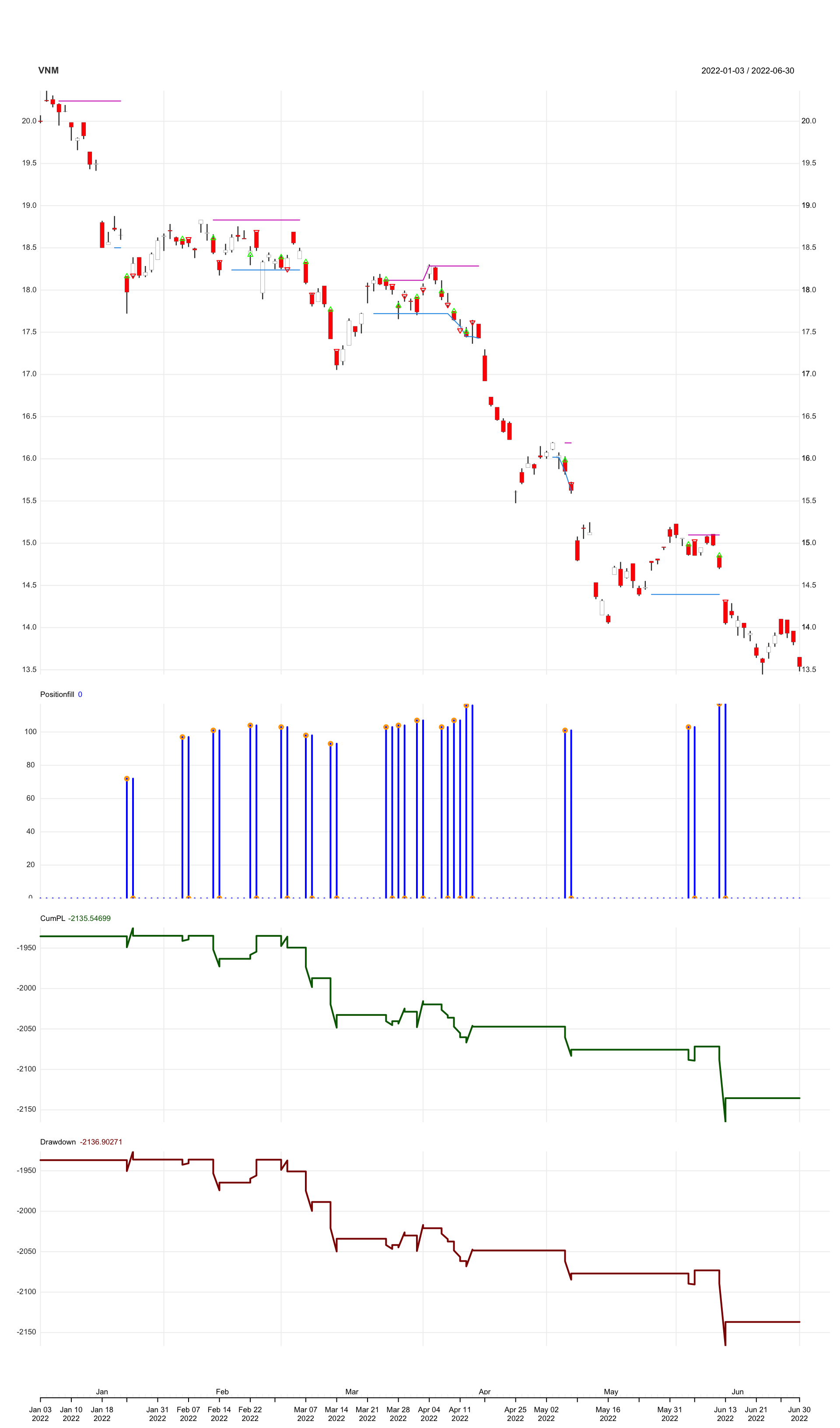
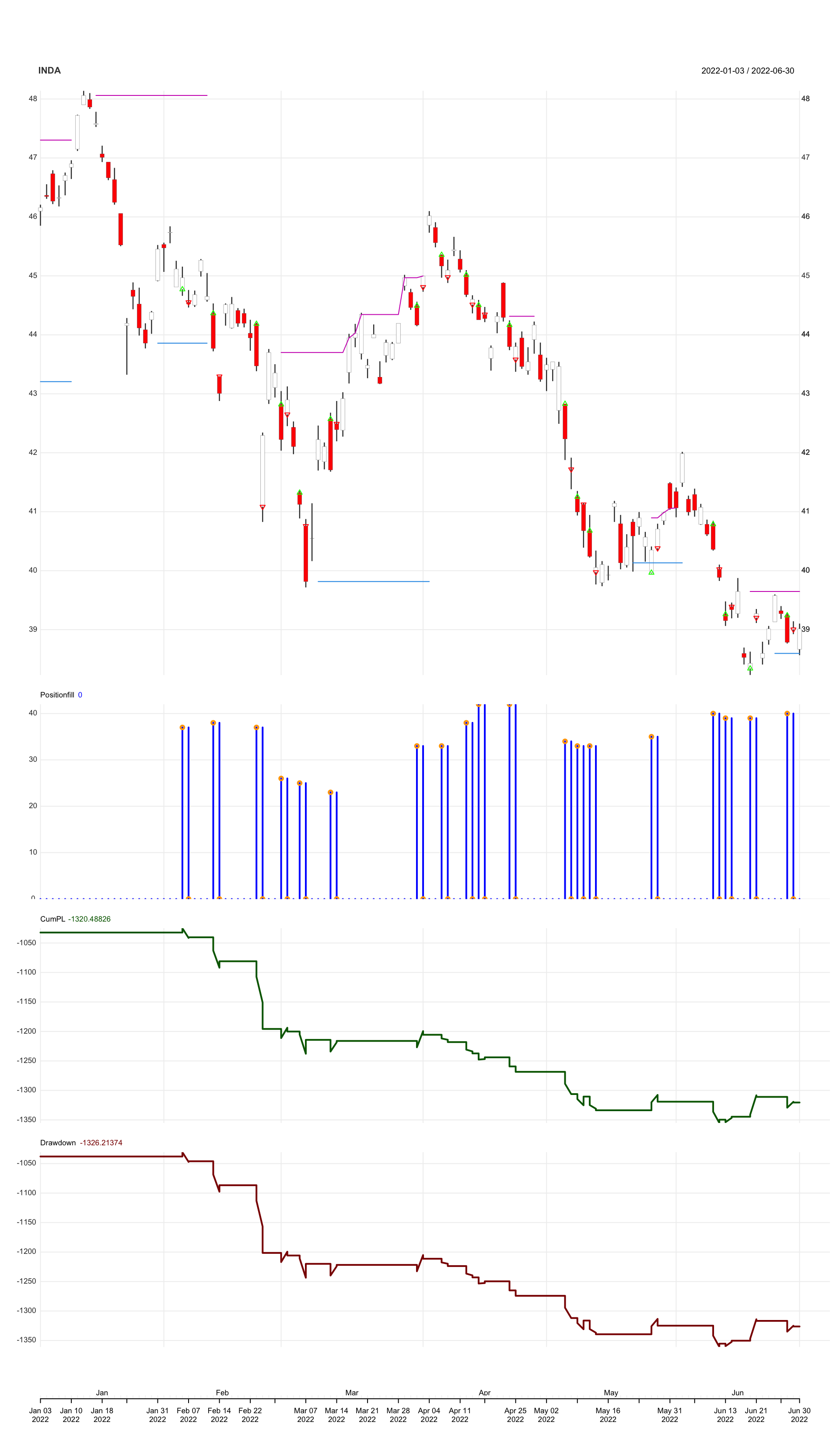
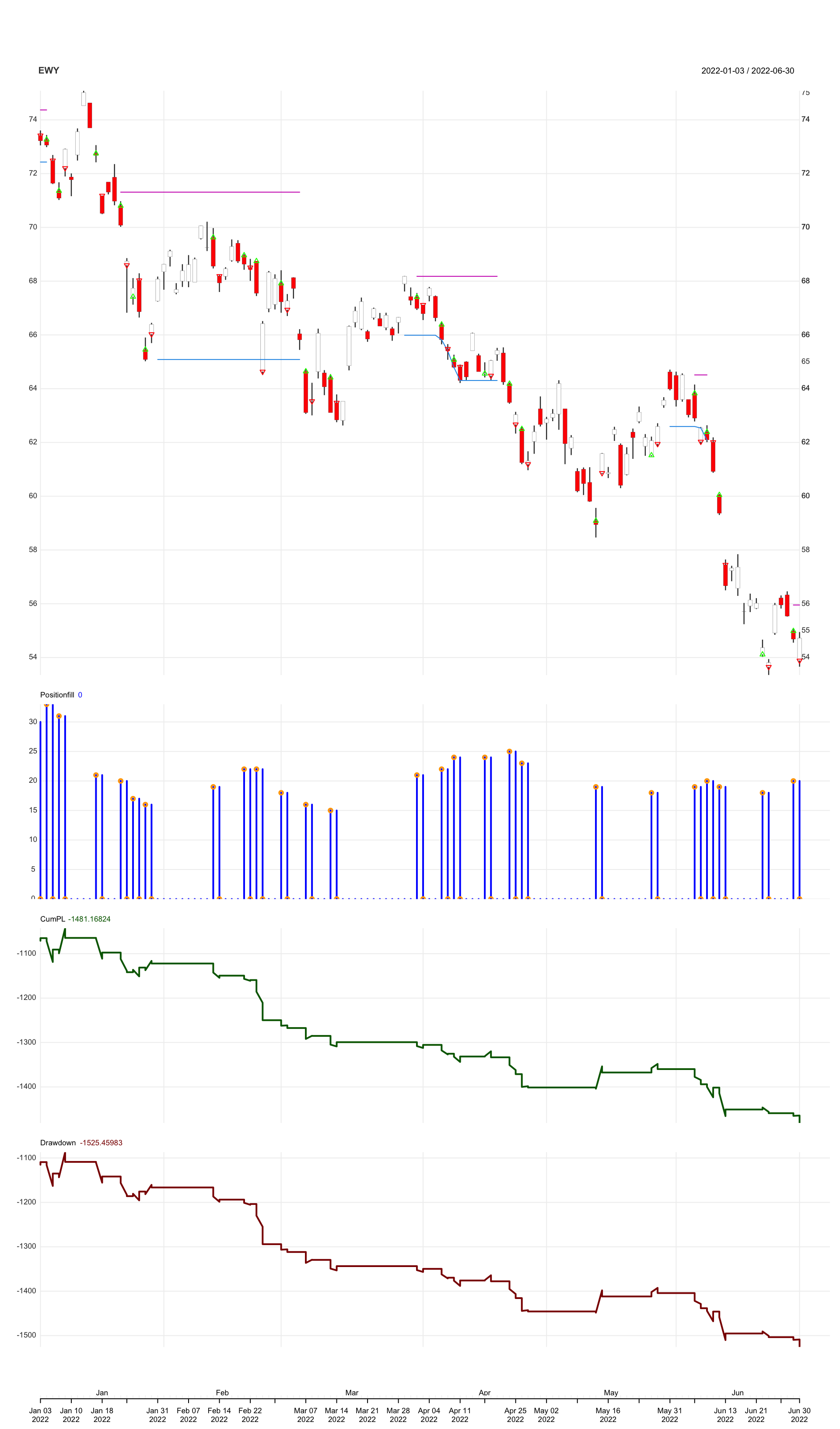
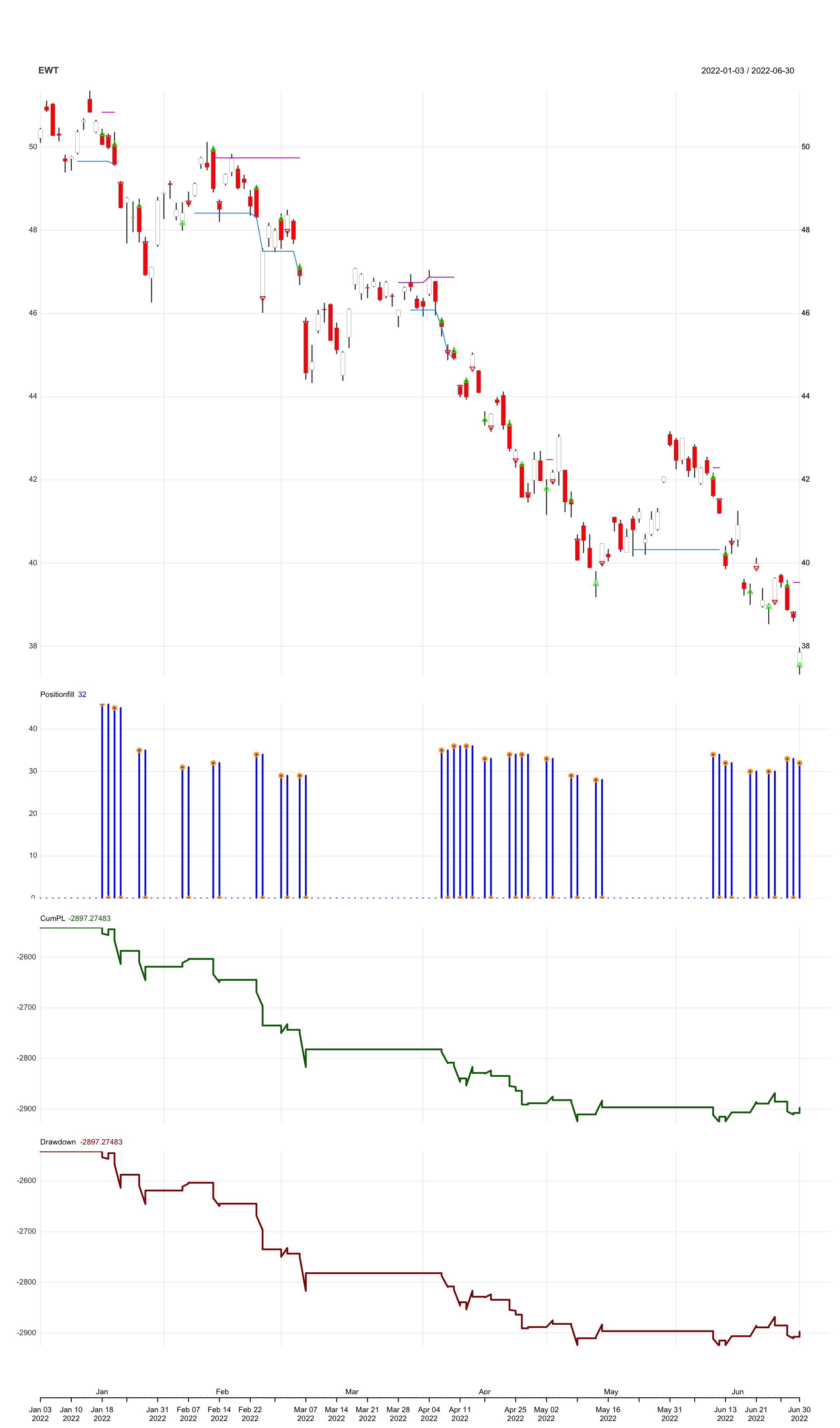
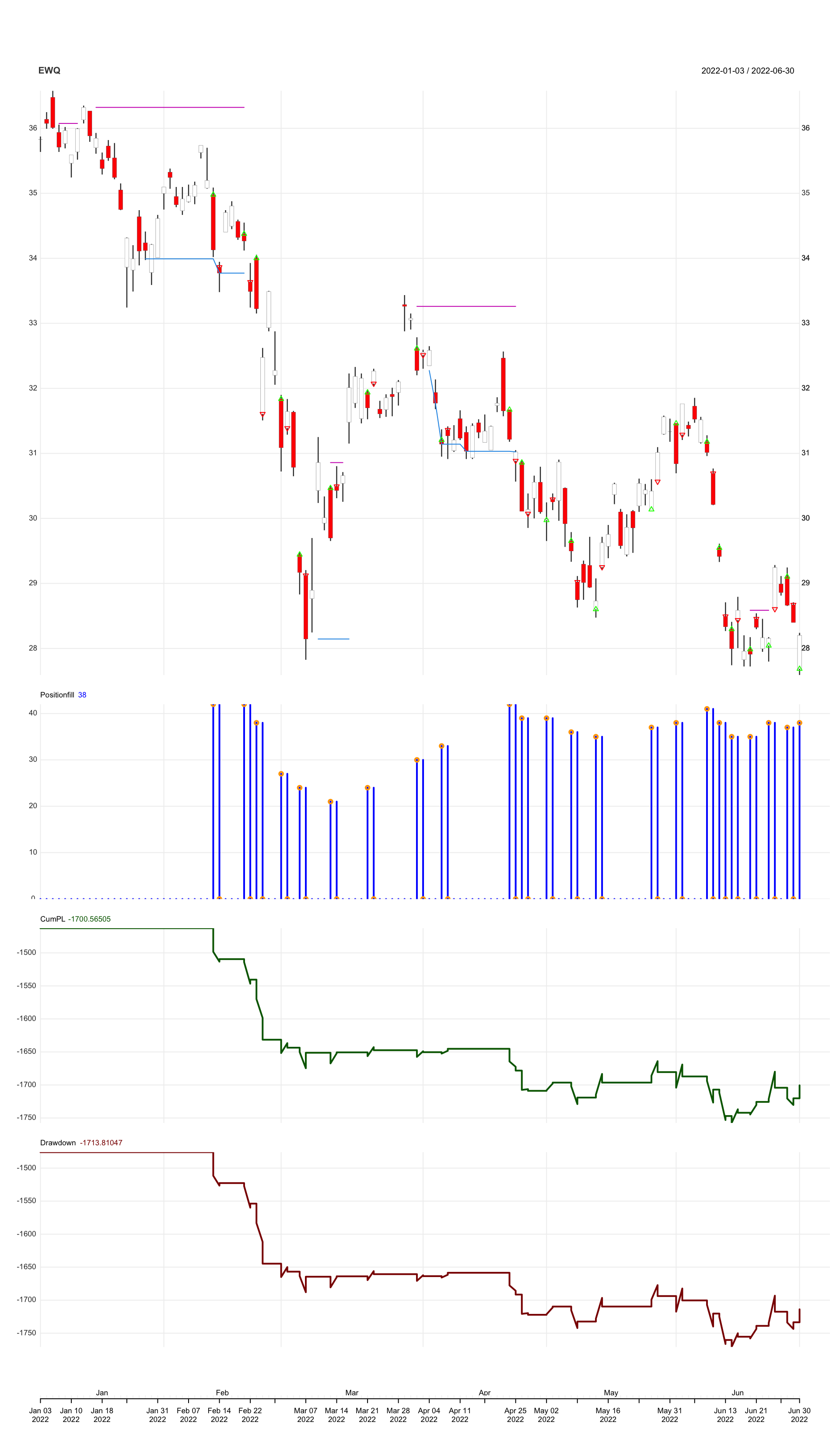
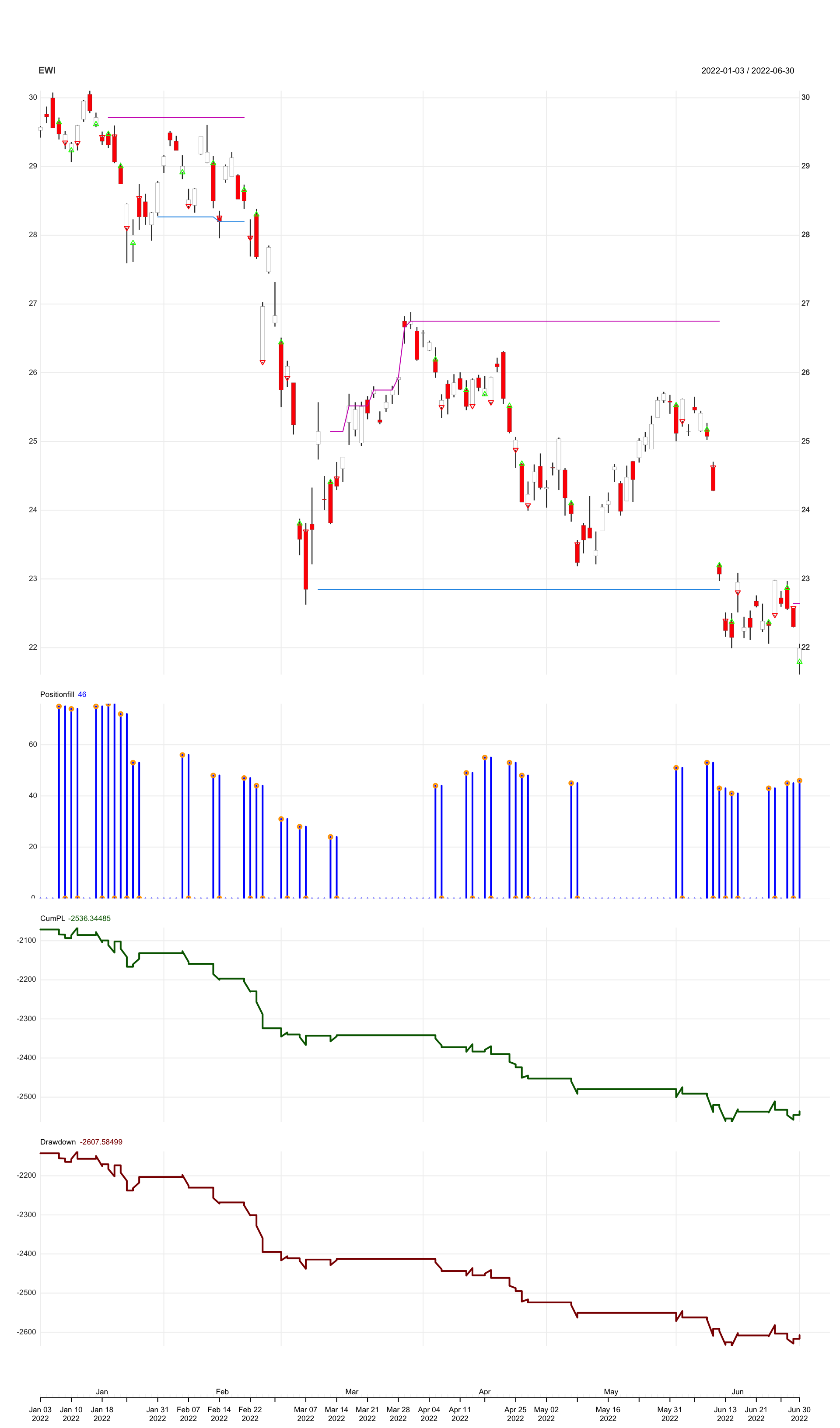
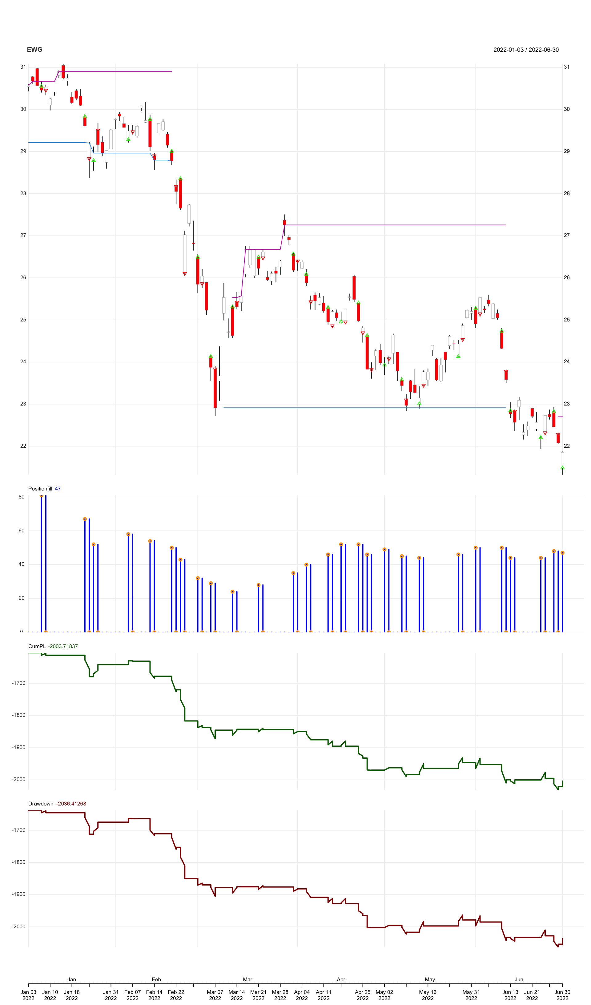
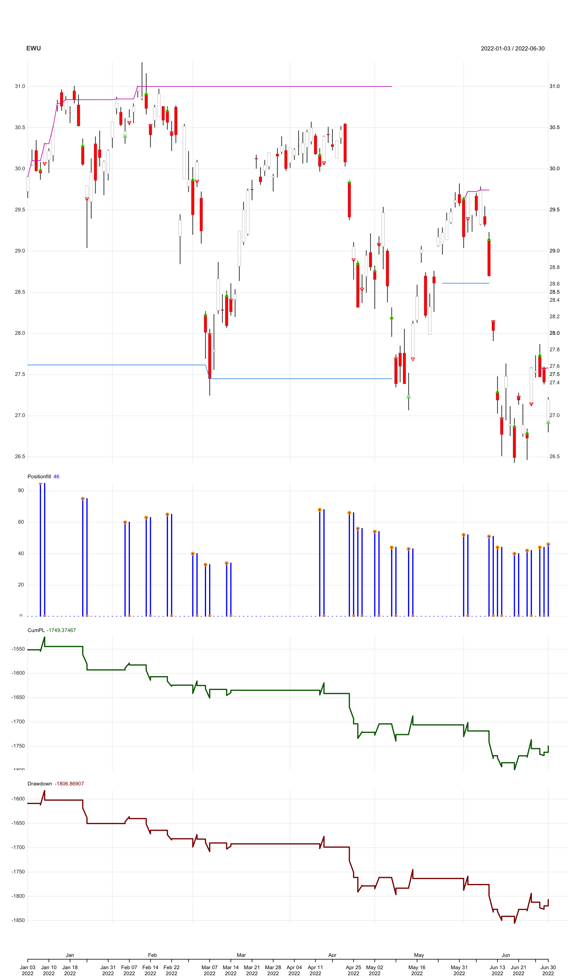
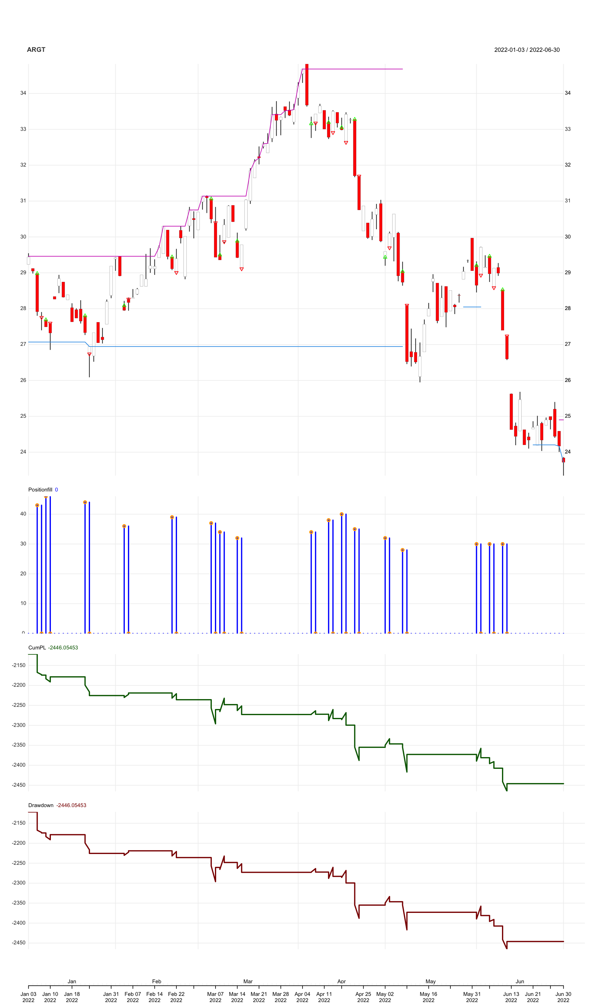
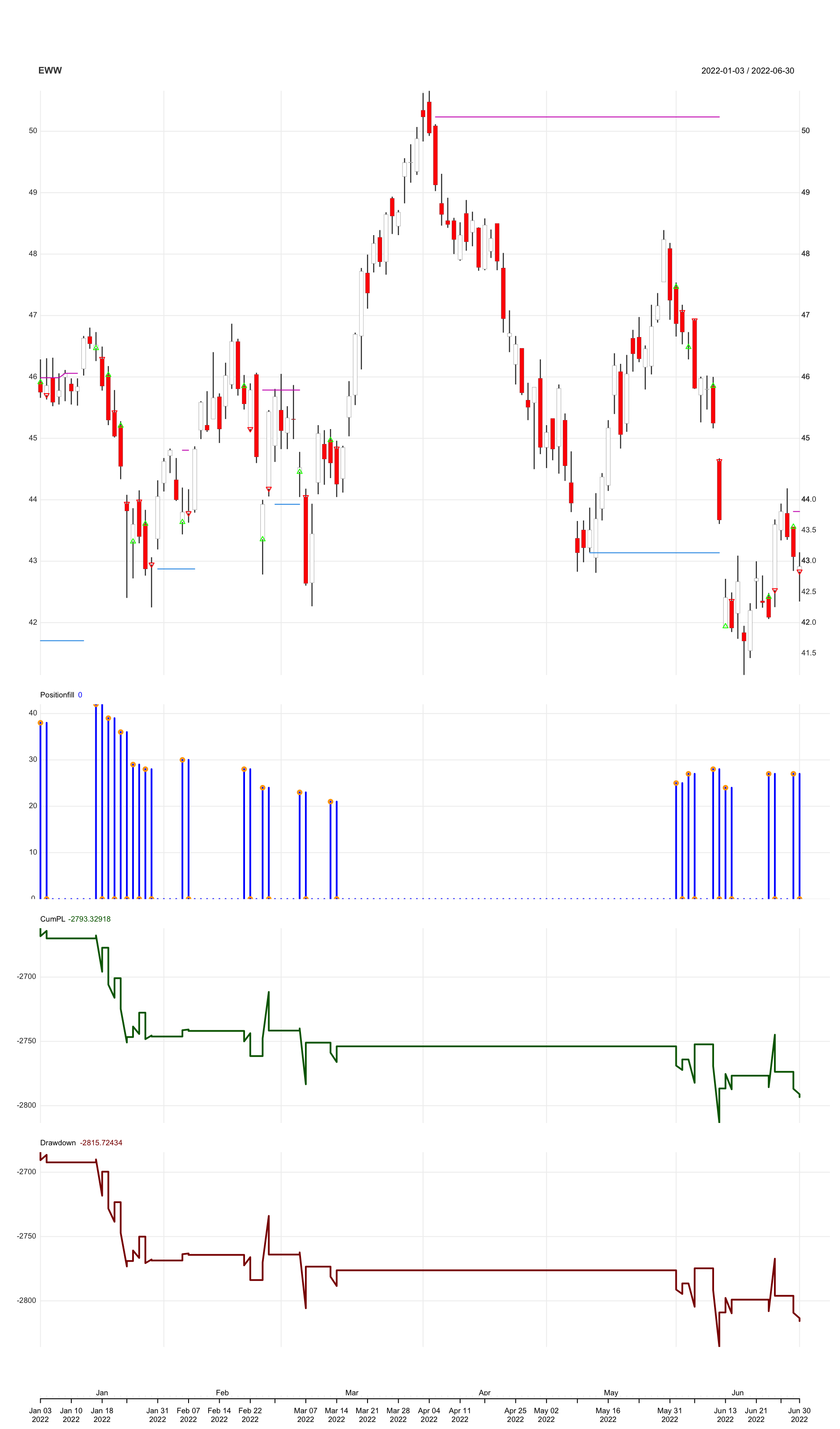
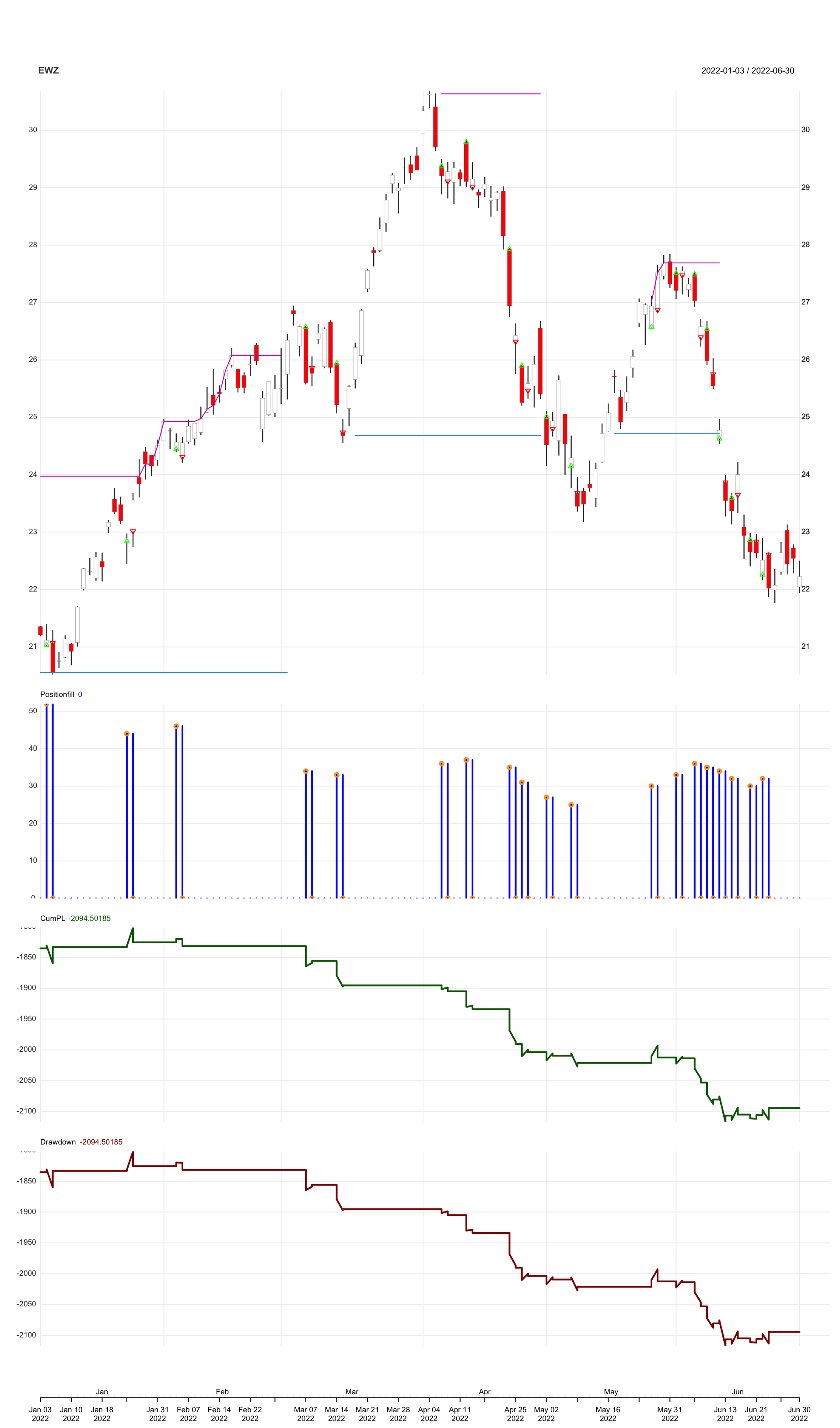
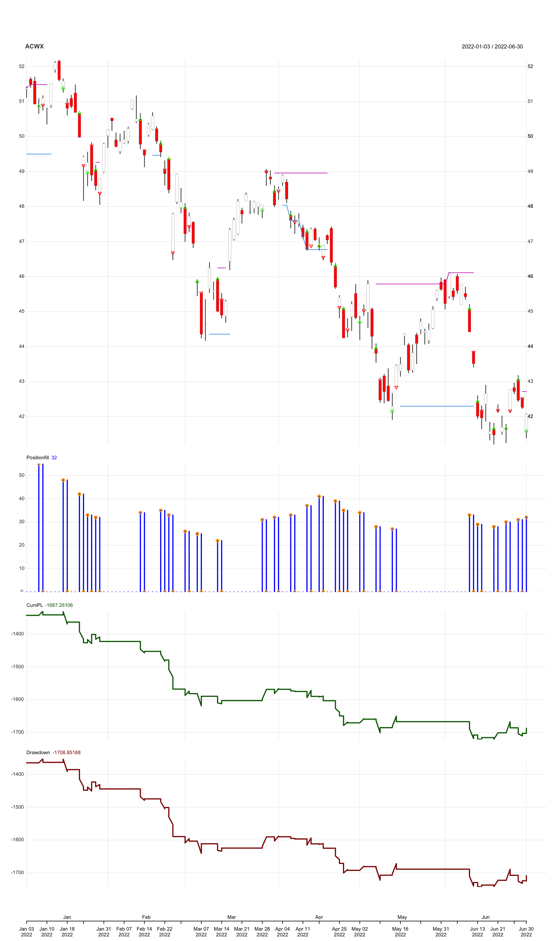
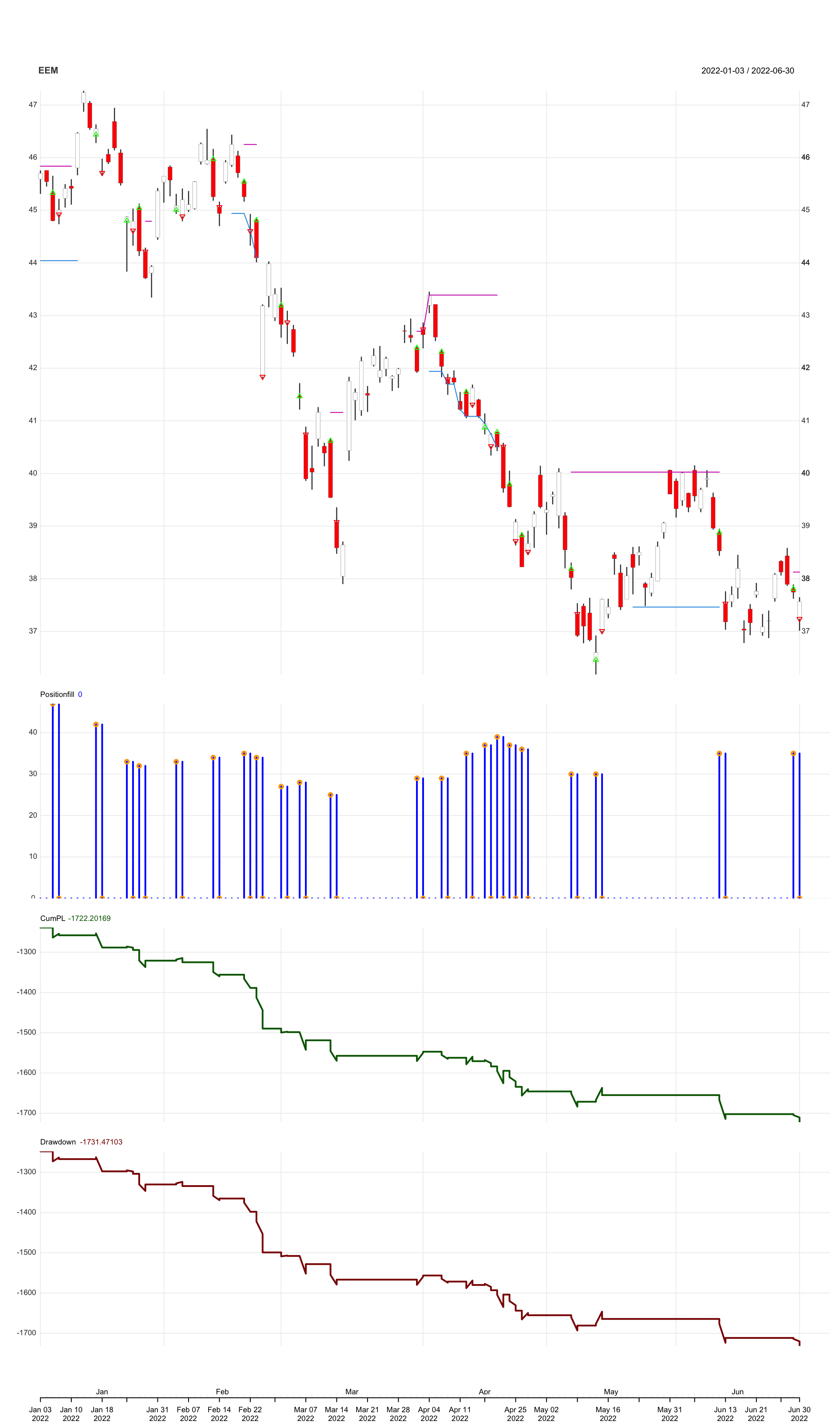
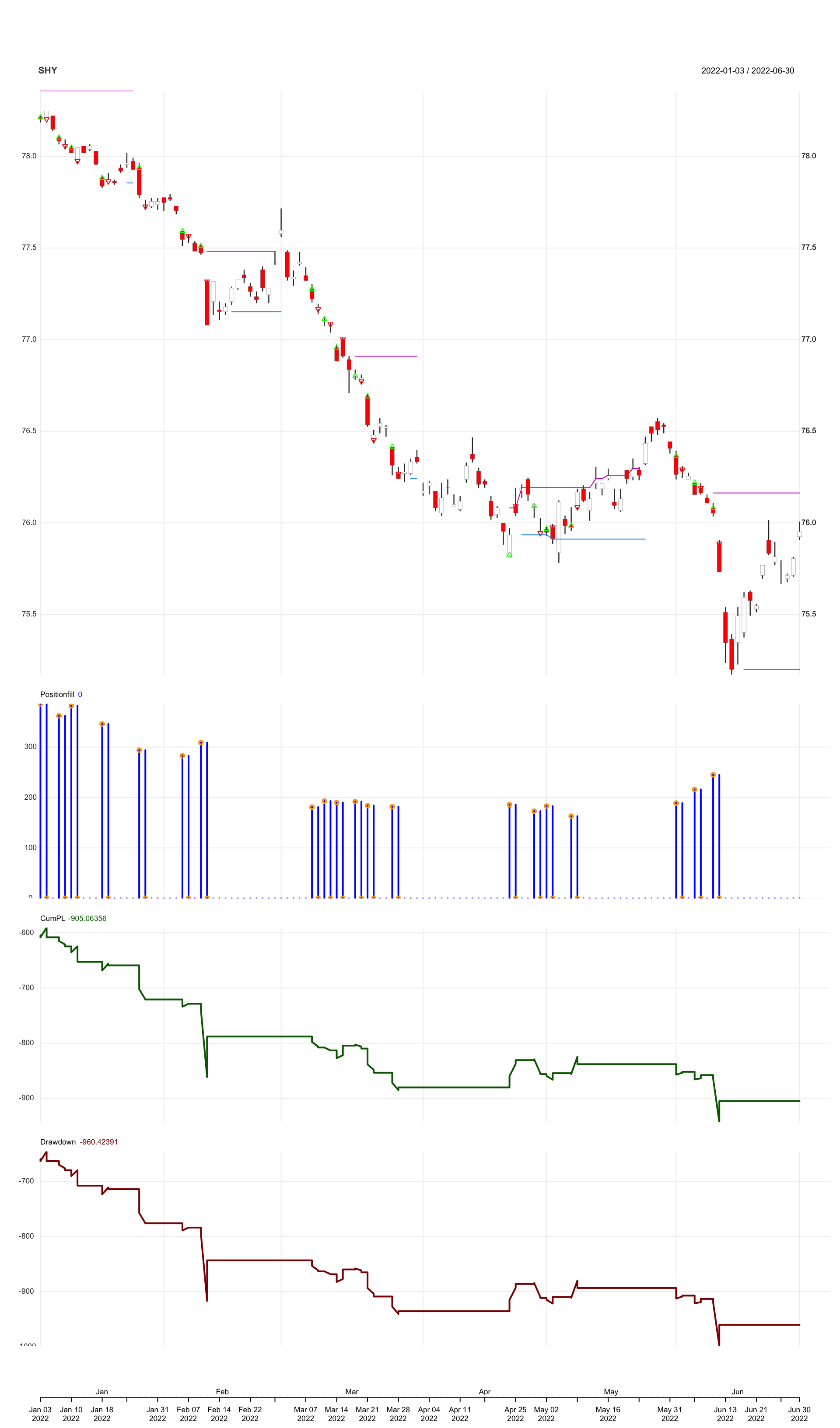
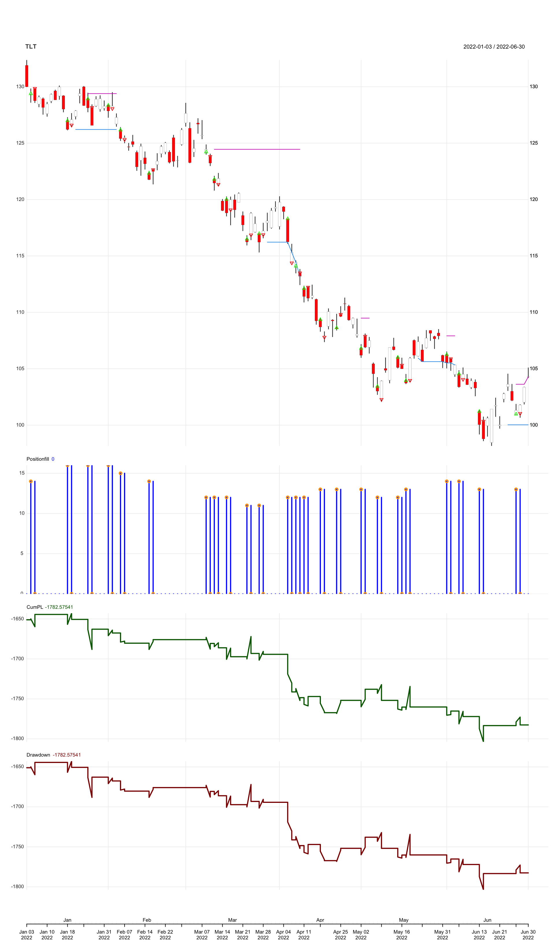
Notes
I think this system is overly-complicated and there are a lot of rules in defining the congestion zone. Due to the limitation of quantstrat, it is not possible to open the position at Open and close the position at Close. I took the alternative to hold it for whole day and close at the next day Open, and by visual inspection, most of the close are not ideal. The results are very bad as well.
For the next steps, it is also required to develop the position sizing strategy for Futures. Let’s put it to a close here as it doesn’t worth to spend more time on this system.